tedana’s denoising approach

tedana works by decomposing multi-echo BOLD data via principal component analysis (PCA) and independent component analysis (ICA). The resulting components are then analyzed to determine whether they are TE-dependent or -independent. TE-dependent components are classified as BOLD, while TE-independent components are classified as non-BOLD, and are discarded as part of data cleaning.

In tedana, we take the time series from all the collected TEs, combine them, and decompose the resulting data into components that can be classified as BOLD or non-BOLD. This is performed in a series of steps, including:

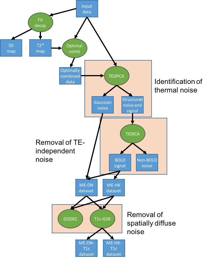
We provide more detail on each step below. The figures shown in this walkthrough are generated in the provided notebooks.

Multi-echo data 

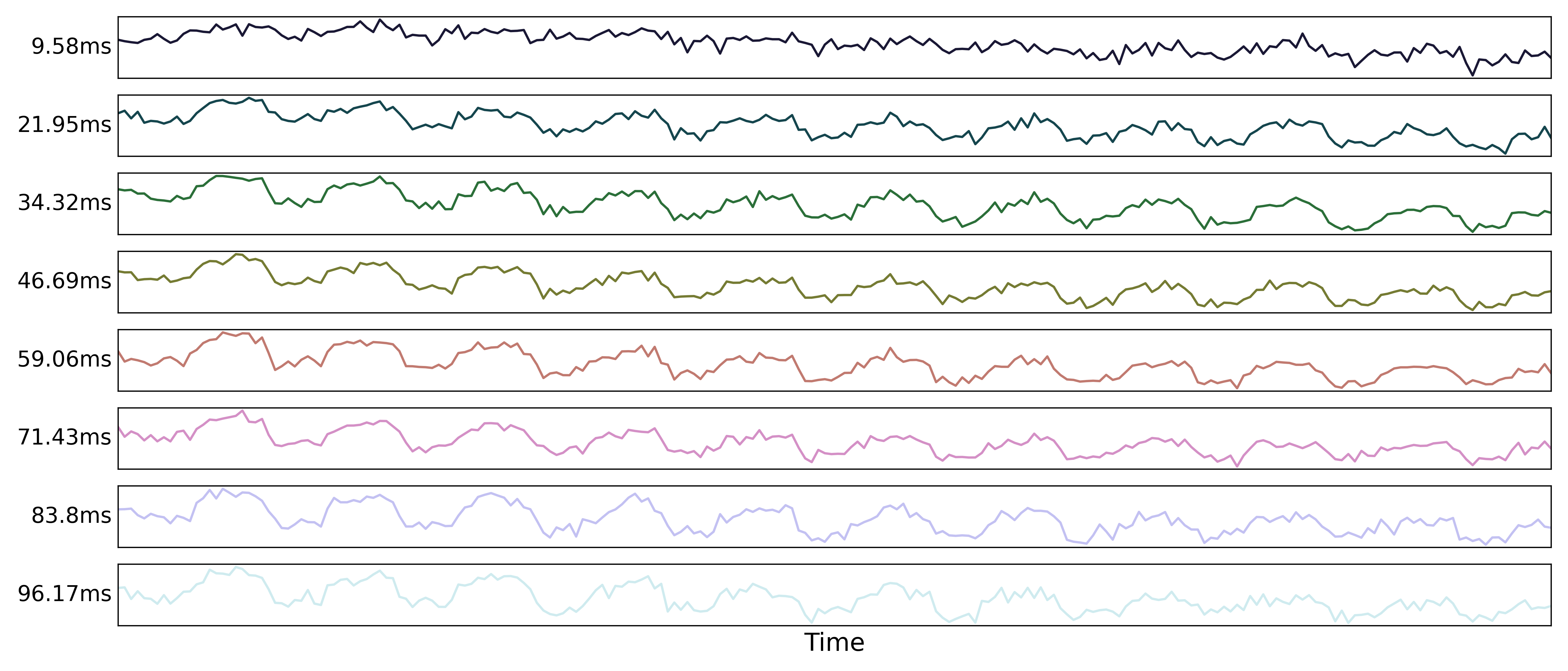
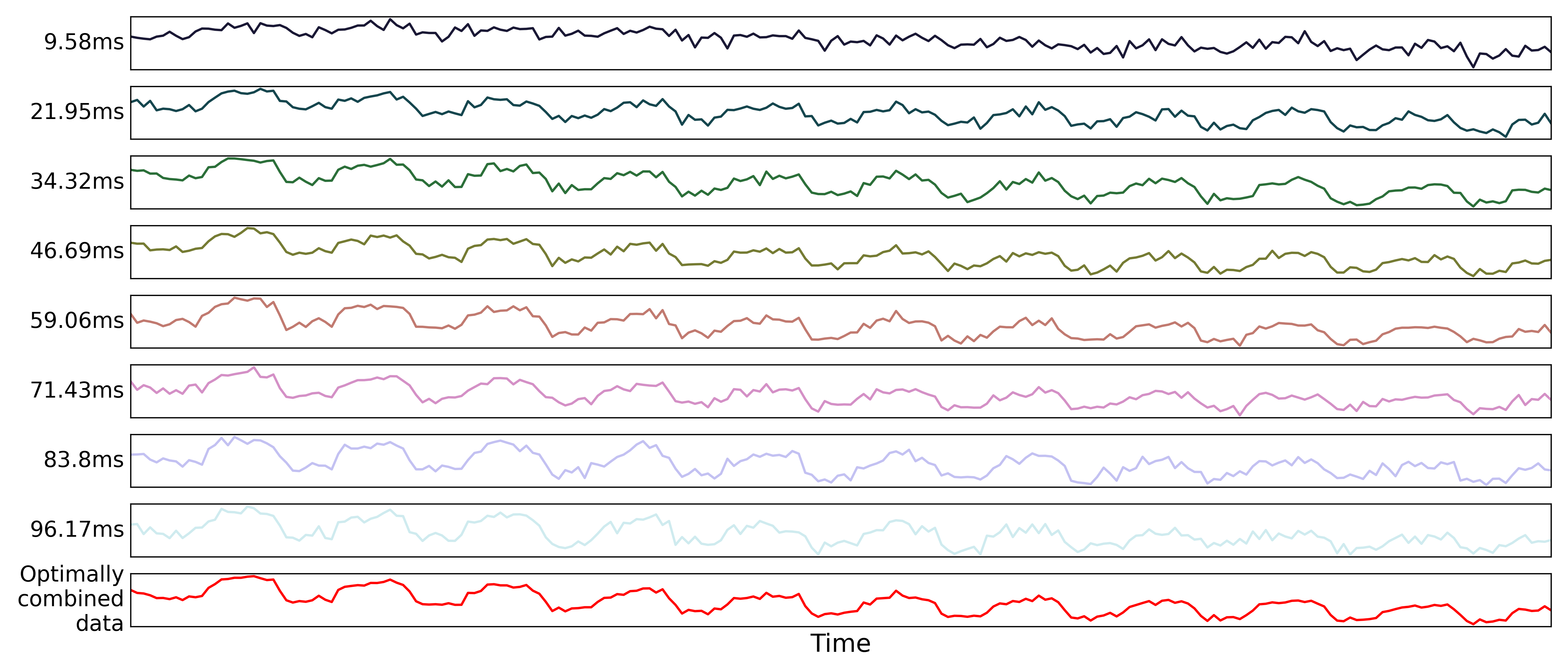
Here are the echo-specific time series for a single voxel in an example resting-state scan with 8 echoes.

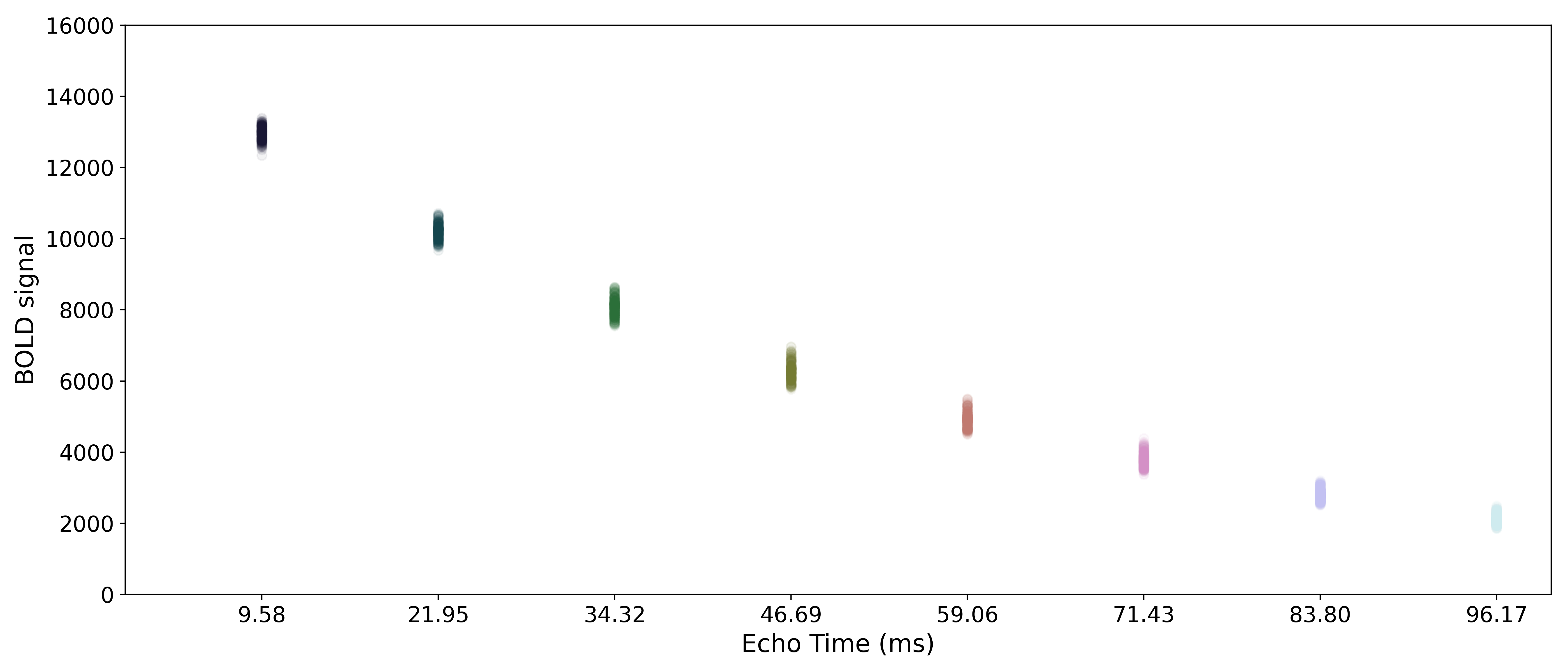
The values across volumes for this voxel scale with echo time in a predictable manner.

_images/a02_echo_value_distributions.png

Adaptive mask generation 

tedana.utils.make_adaptive_mask()

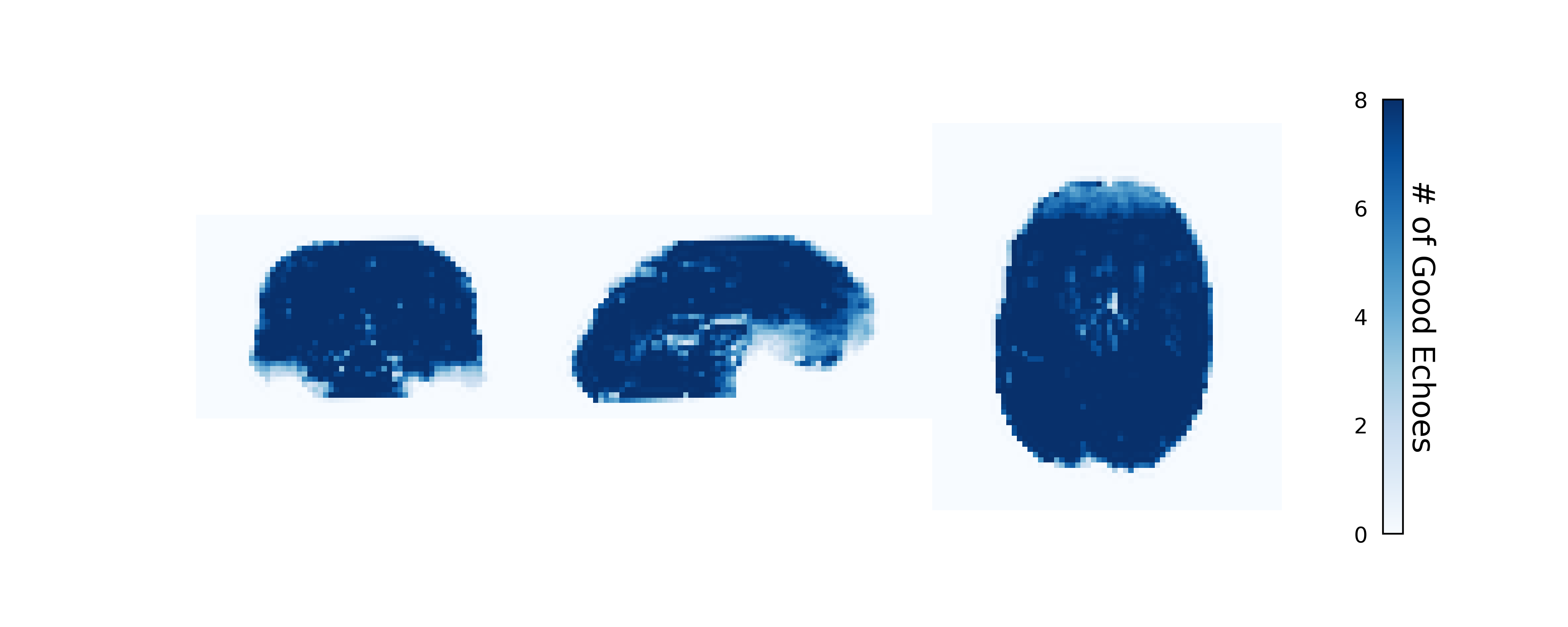
Longer echo times are more susceptible to signal dropout, which means that certain brain regions (e.g., orbitofrontal cortex, temporal poles) will only have good signal for some echoes. In order to avoid using bad signal from affected echoes in calculating $T_{2}^*$ and $S_{0}$ for a given voxel, tedana generates an adaptive mask, where the value for each voxel is the number of echoes with “good” signal. When $T_{2}^*$ and $S_{0}$ are calculated below, each voxel’s values are only calculated from the first $n$ echoes, where $n$ is the value for that voxel in the adaptive mask.

Note

tedana allows users to provide their own mask. The adaptive mask will be computed on this explicit mask, and may reduce it further based on the data. If a mask is not provided, tedana runs nilearn.masking.compute_epi_mask() on the first echo’s data to derive a mask prior to adaptive masking. The workflow does this because the adaptive mask generation function sometimes identifies almost the entire bounding box as “brain”, and compute_epi_mask restricts analysis to a more reasonable area.

Monoexponential decay model fit 

tedana.decay.fit_decay()

The next step is to fit a monoexponential decay model to the data in order to estimate voxel-wise $T_{2}^*$ and $S_0$ . $S_0$ corresponds to the total signal in each voxel before decay and can reflect coil sensivity. $T_{2}^*$ corresponds to the rate at which a voxel decays over time, which is related to signal dropout and BOLD sensitivity. Estimates of the parameters are saved as T2starmap.nii.gz and S0map.nii.gz.

While $T_{2}^*$ and $S_0$ in fact fluctuate over time, estimating them on a volume-by-volume basis with only a small number of echoes is not feasible (i.e., the estimates would be extremely noisy). As such, we estimate average $T_{2}^*$ and $S_0$ maps and use those throughout the workflow.

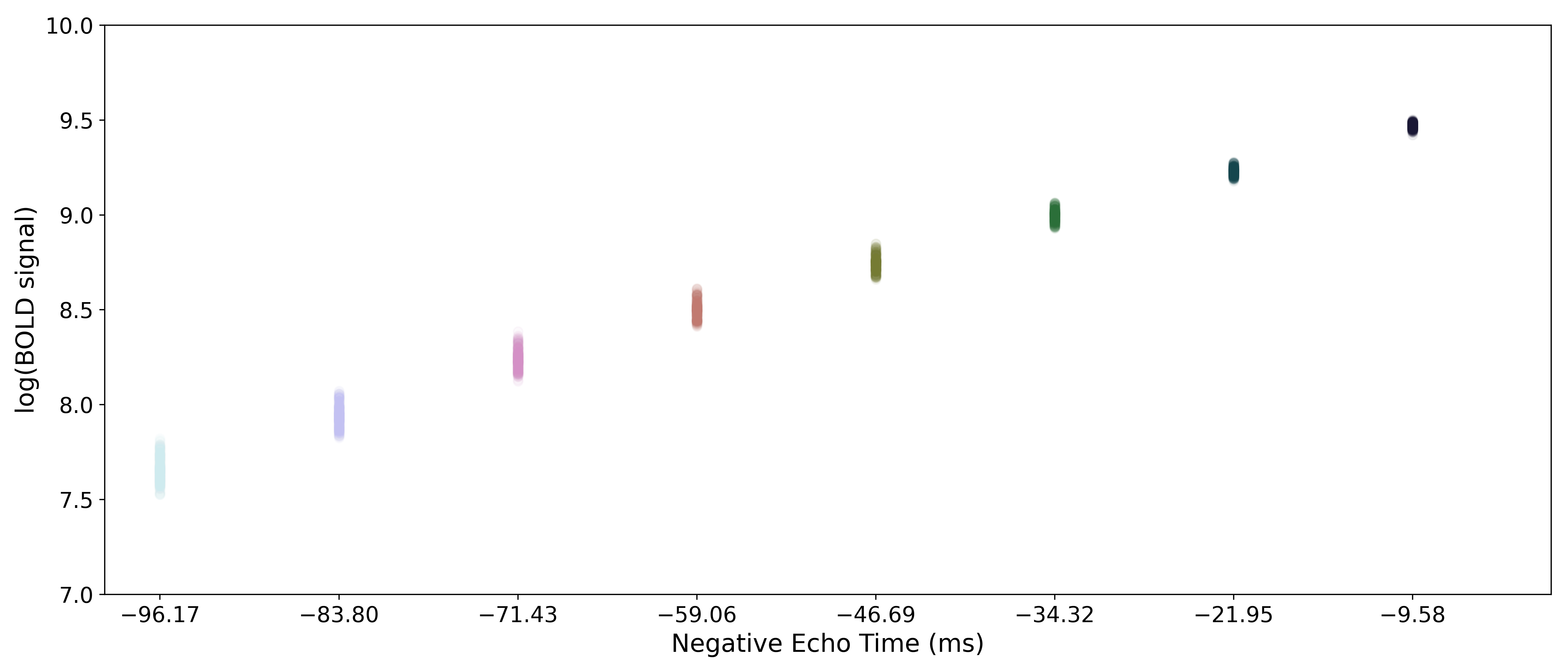
In order to make it easier to fit the decay model to the data, tedana transforms the data by default. The BOLD data are transformed as $log(|S|+1)$ , where $S$ is the BOLD signal. The echo times are also multiplied by -1.

Tip

It is now possible to do a nonlinear monoexponential fit to the original, untransformed data values by specifiying --fittype curvefit. This method is slightly more computationally demanding but may obtain more accurate fits.

_images/a04_echo_log_value_distributions.png

A simple line can then be fit to the transformed data with linear regression. For the sake of this introduction, we can assume that the example voxel has good signal in all eight echoes (i.e., the adaptive mask has a value of 8 at this voxel), so the line is fit to all available data.

Note

tedana actually performs and uses two sets of $T_{2}^*$ / $S_0$ model fits. In one case, tedana estimates $T_{2}^*$ and $S_0$ for voxels with good signal in at least two echoes. In the other case, tedana estimates $T_{2}^*$ and $S_0$ for voxels with good data in only one echo as well, but uses the first two echoes for those voxels. The resulting “full” $T_{2}^*$ and $S_0$ maps are used throughout the rest of the pipeline.

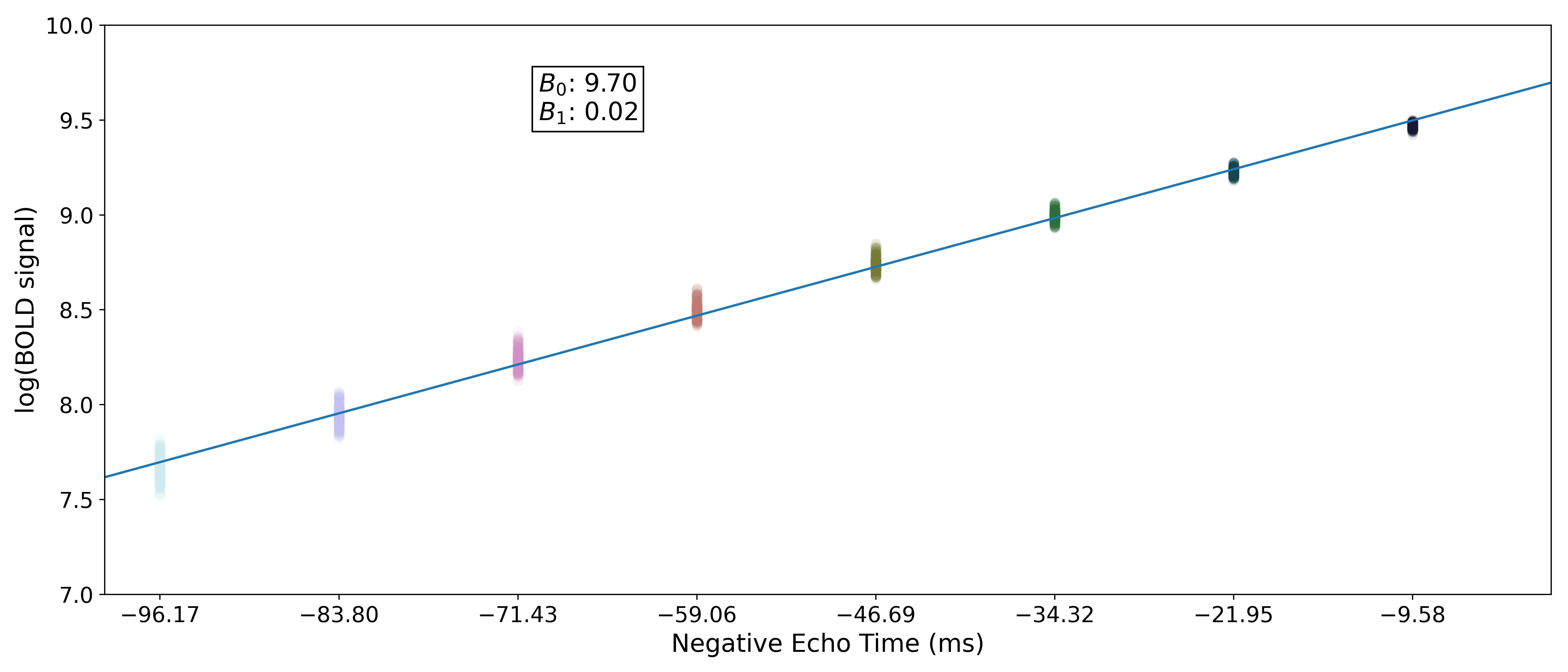
The values of interest for the decay model, $S_0$ and $T_{2}^*$ , are then simple transformations of the line’s intercept ( $B_{0}$ ) and slope ( $B_{1}$ ), respectively:

$S_{0} = e^{B_{0}}$

$T_{2}^{*} = \frac{1}{B_{1}}$

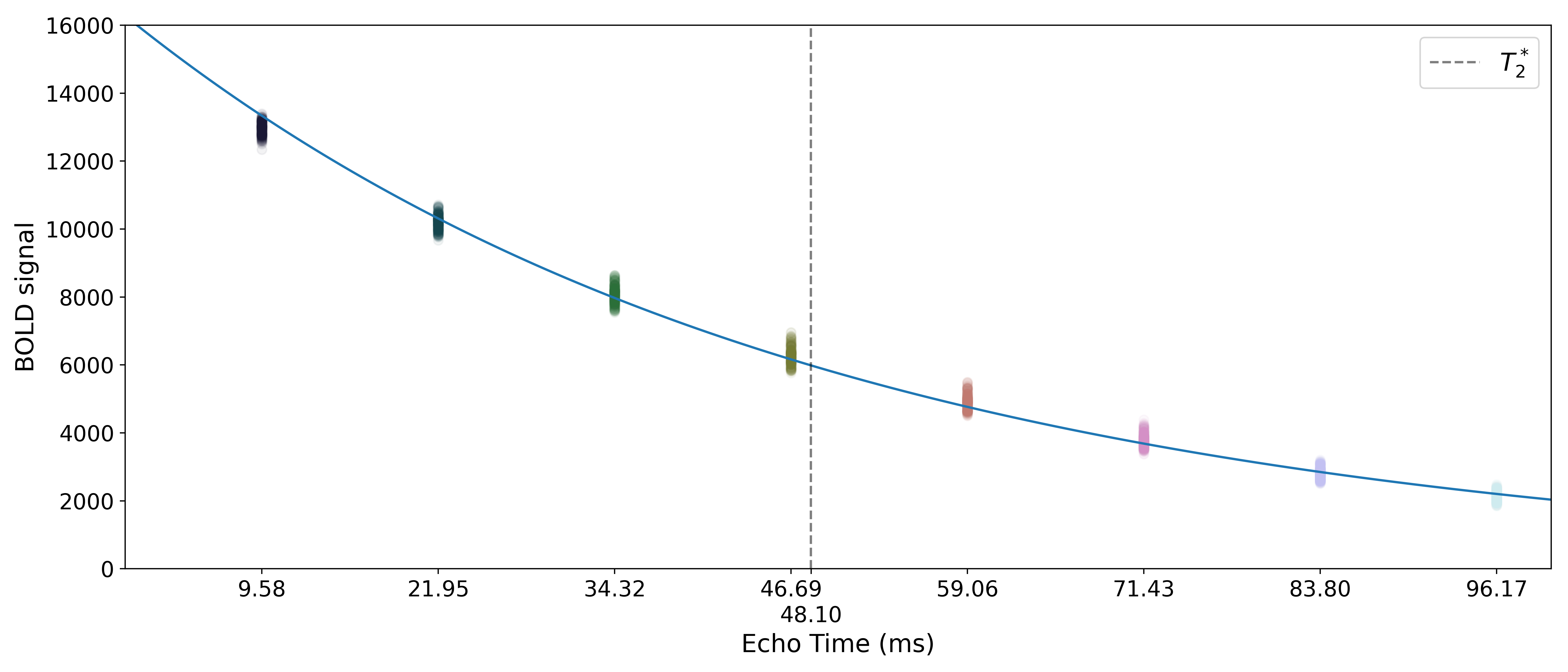
The resulting values can be used to show the fitted monoexponential decay model on the original data.

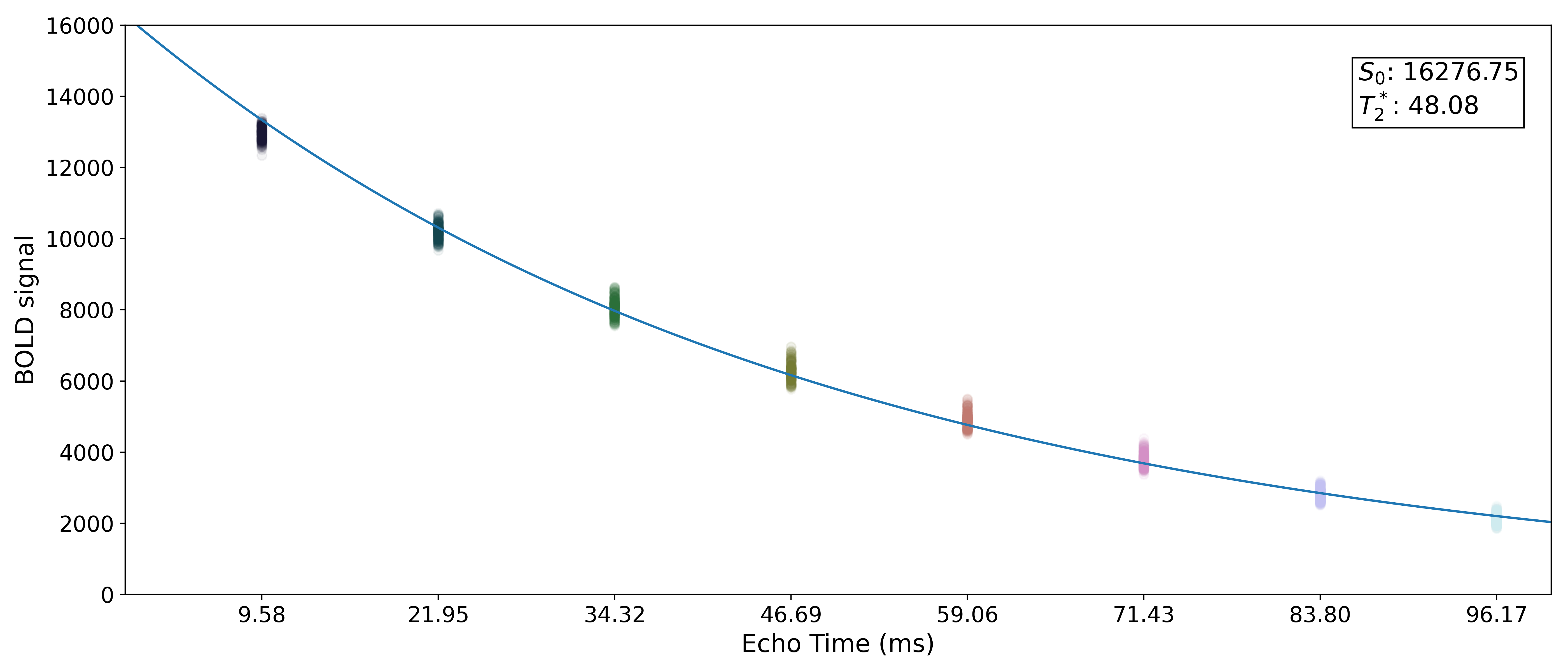
_images/a06_monoexponential_decay_model.png

We can also see where $T_{2}^*$ lands on this curve.

_images/a07_monoexponential_decay_model_with_t2.png

Optimal combination 

tedana.combine.make_optcom()

Using the $T_{2}^*$ estimates, tedana combines signal across echoes using a weighted average. The echoes are weighted according to the formula

$w_{TE} = TE * e^{\frac{-TE}{T_{2}^*}}$

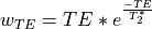
The weights are then normalized across echoes. For the example voxel, the resulting weights are:

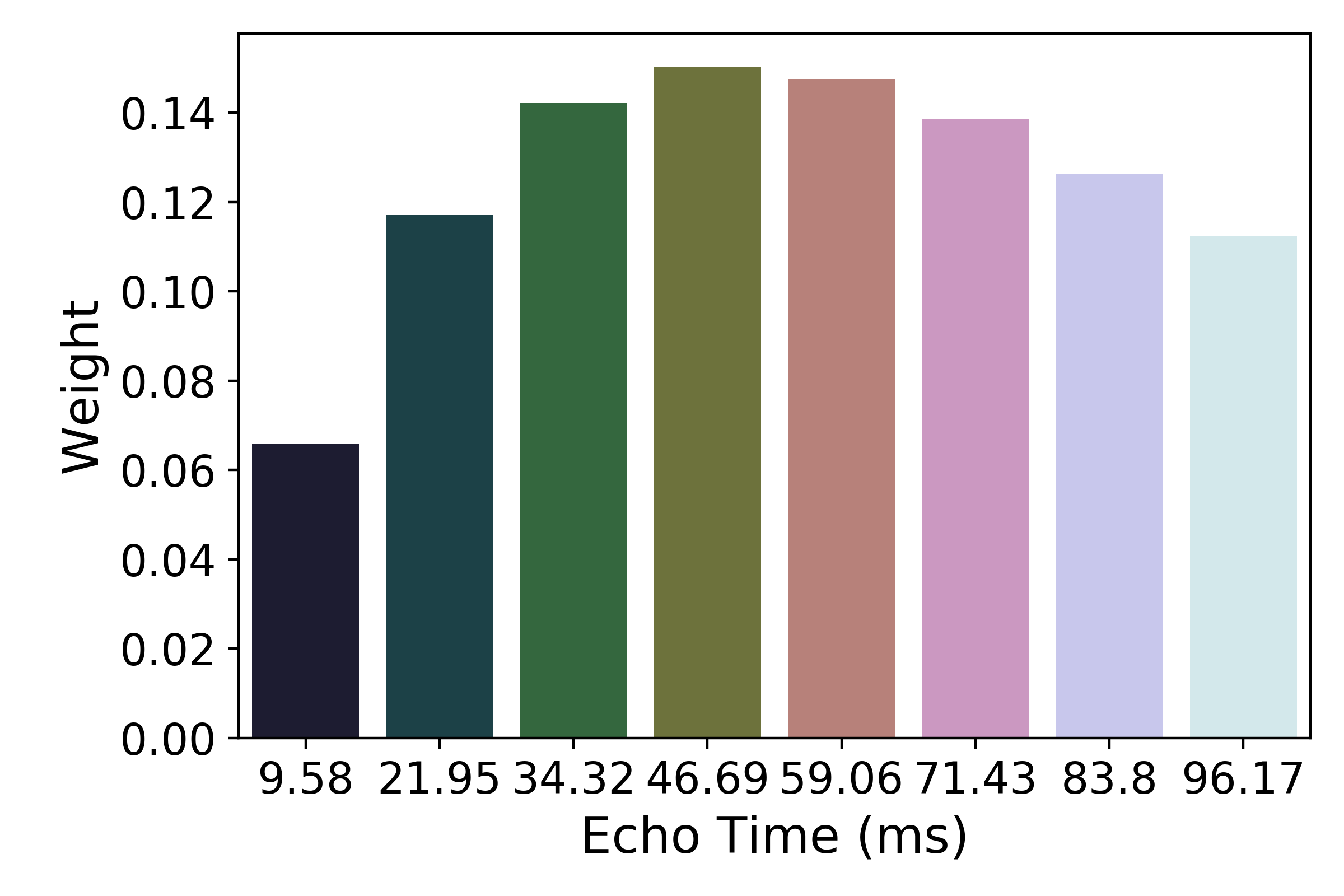
_images/a08_optimal_combination_echo_weights.png

These normalized weights are then used to compute a weighted average that takes advantage of the higher signal in earlier echoes and the higher sensitivity at later echoes. The distribution of values for the optimally combined data lands somewhere between the distributions for other echoes.

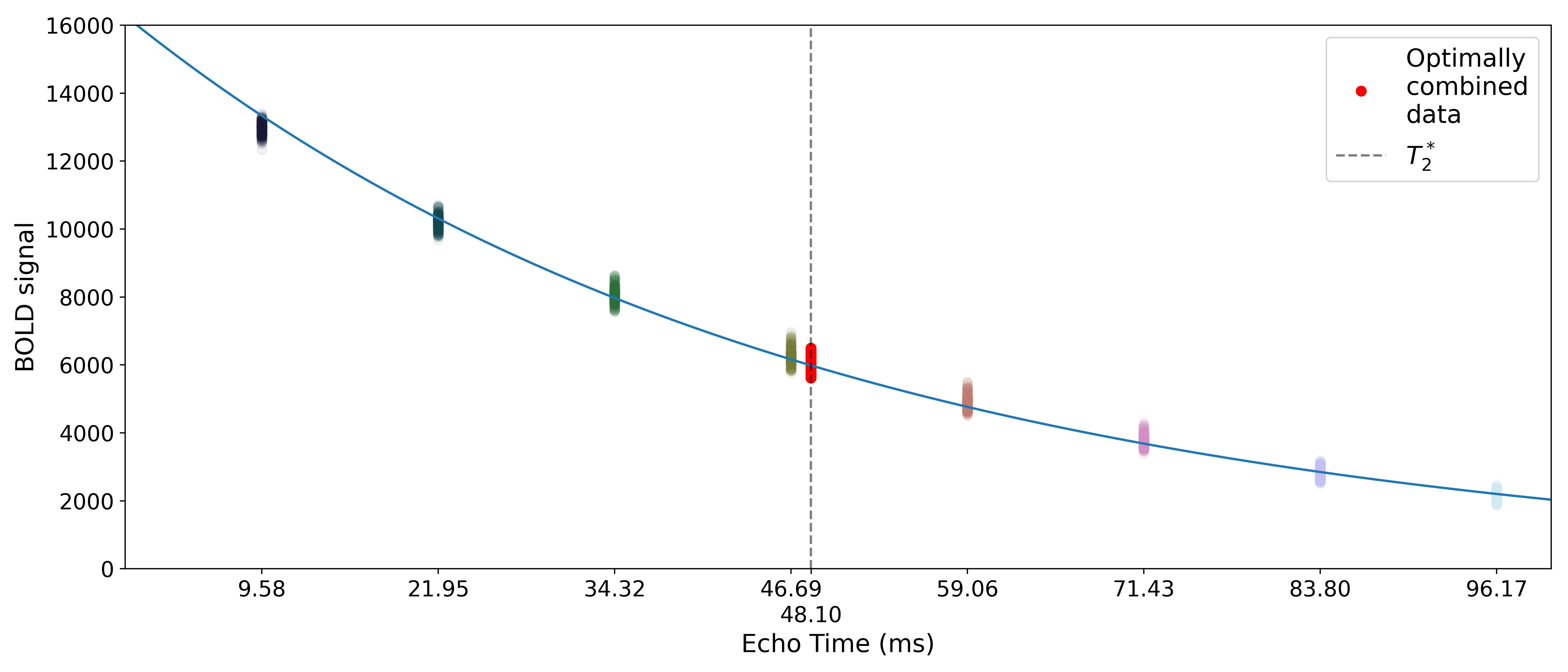
_images/a09_optimal_combination_value_distributions.png

The time series for the optimally combined data also looks like a combination of the other echoes (which it is). This optimally combined data is written out as desc-optcom_bold.nii.gz

_images/a10_optimal_combination_timeseries.png

Note

An alternative method for optimal combination that does not use $T_{2}^*$ is the parallel-acquired inhomogeneity desensitized (PAID) ME-fMRI combination method (Poser et al., 2006). This method specifically assumes that noise in the acquired echoes is “isotopic and homogeneous throughout the image,” meaning it should be used on smoothed data. As we do not recommend performing tedana denoising on smoothed data, we discourage using PAID within the tedana workflow. We do, however, make it accessible as an alternative combination method in tedana.workflows.t2smap_workflow().

Denoising 

The next step is an attempt to remove noise from the data. This process can be broadly separated into three steps: decomposition, metric calculation and component selection. Decomposition reduces the dimensionality of the optimally combined data using principal component analysis (PCA) and then an independent component analysis (ICA). Metrics that evaluate TE-dependence or independence are derived from these components. Component selection uses these metrics in order to identify components that should be kept in the data or discarded. Unwanted components are then removed from the optimally combined data to produce the denoised data output.

TEDPCA 

tedana.decomposition.tedpca()

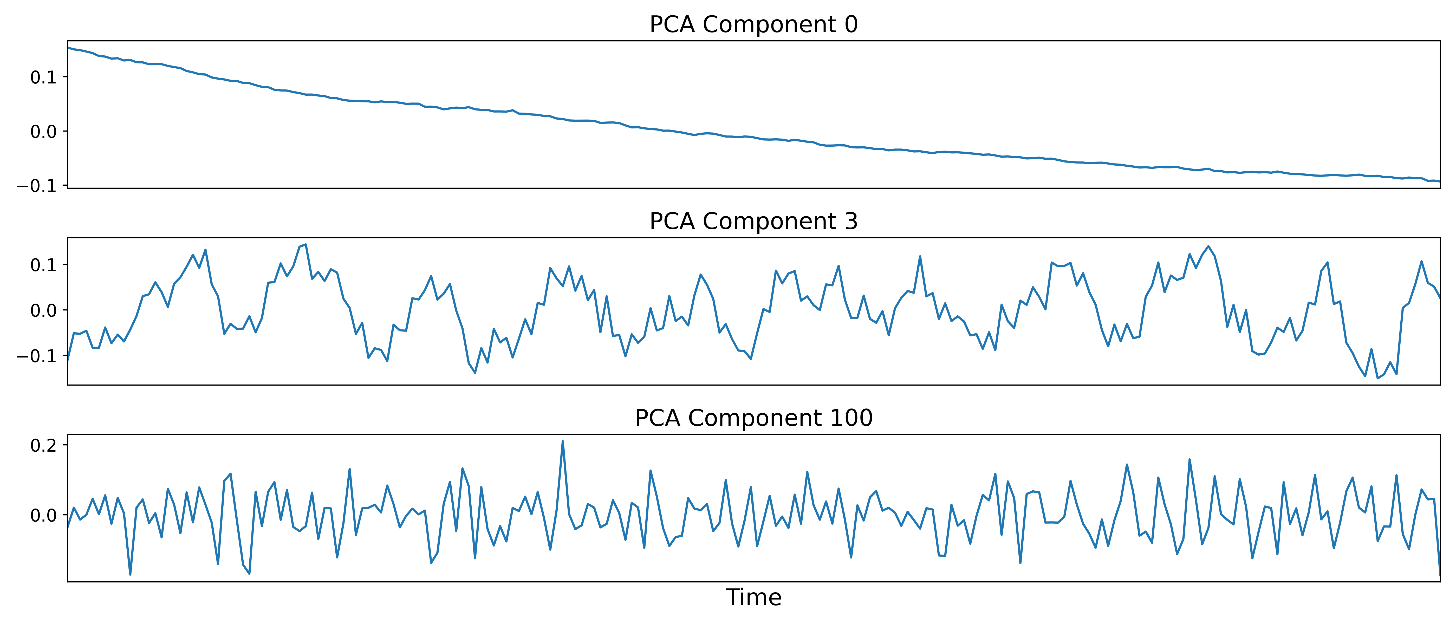
The next step is to dimensionally reduce the data with TE-dependent principal component analysis (PCA). The goal of this step is to make it easier for the later ICA decomposition to converge. Dimensionality reduction is a common step prior to ICA. TEDPCA applies PCA to the optimally combined data in order to decompose it into component maps and time series (saved as desc-PCA_mixing.tsv). Here we can see time series for some example components (we don’t really care about the maps):

_images/a11_pca_component_timeseries.png

These components are subjected to component selection, the specifics of which vary according to algorithm. Specifically, tedana offers three different approaches that perform this step.

The recommended approach (the default aic option, along with the kic and mdl options, for --tedpca) is based on a moving average (stationary Gaussian) process proposed by Li et al (2007) and used primarily in the Group ICA of fMRI Toolbox (GIFT). A moving average process is the output of a linear system (which, in this case, is a smoothing filter) that has an independent and identically distributed Gaussian process as the input. Simply put, this process more optimally selects the number of components for fMRI data following a subsampling scheme described in Li et al (2007).

The number of selected principal components depends on the selection criteria. For this PCA method in particular, --tedpca provides three different options to select the PCA components based on three widely-used model selection criteria:

mdl: the Minimum Description Length (MDL), which is the most aggressive option; i.e. returns the least number of components.
kic: the Kullback-Leibler Information Criterion (KIC), which stands in the middle in terms of aggressiveness. You can see how KIC is related to AIC here.
aic: the Akaike Information Criterion (AIC), which is the least aggressive option; i.e., returns the largest number of components. We have chosen AIC as the default PCA criterion because it tends to result in fewer components than the Kundu methods, which increases the likelihood that the ICA step will successfully converge, but also, in our experience, retains enough components for meaningful interpretation later on.

Note

Please, bear in mind that this is a data-driven dimensionality reduction approach. The default option aic might not yield perfect results on your data. Consider kic and mdl options if running tedana with aic returns more components than expected. There is no definitively right number of components, but, for typical fMRI datasets, if the PCA explains more than 98% of the variance or if the number of components is more than half the number of time points, then it may be worth considering more aggressive thresholds.

The simplest approach uses a user-supplied threshold applied to the cumulative variance explained by the PCA. In this approach, the user provides a value to --tedpca between 0 and 1. That value corresponds to the percent of variance that must be explained by the components. For example, if a value of 0.9 is provided, then PCA components (ordered by decreasing variance explained) cumulatively explaining up to 90% of the variance will be retained. Components explaining more than that threshold (except for the component that crosses the threshold) will be excluded.

In addition to the moving average process-based options and the variance explained threshold described above, we also support a decision tree-based selection method (similar to the one in the TEDICA section below). This method involves applying a decision tree to identify and discard PCA components which, in addition to not explaining much variance, are also not significantly TE-dependent (i.e., have low Kappa) or TE-independent (i.e., have low Rho). These approaches can be accessed using either the kundu or kundu_stabilize options for the --tedpca flag.

Tip

For more information on how TE-dependence and TE-independence models are estimated in tedana, see TE (In)Dependence Models. For a more thorough explanation of this approach, consider the supplemental information in Kundu et al (2013).

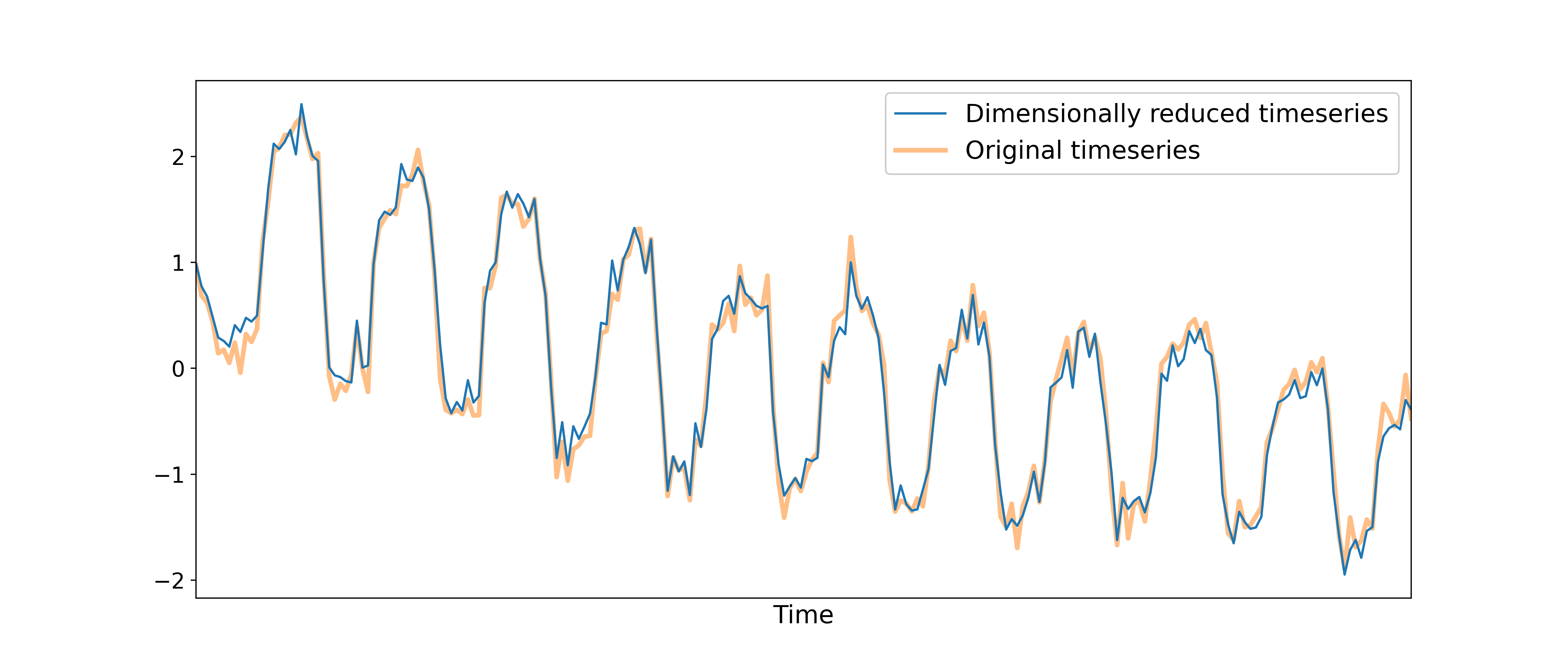
After component selection is performed, the retained components and their associated betas are used to reconstruct the optimally combined data, resulting in a dimensionally reduced version of the dataset which is then used in the TEDICA step.

TEDICA 

tedana.decomposition.tedica()

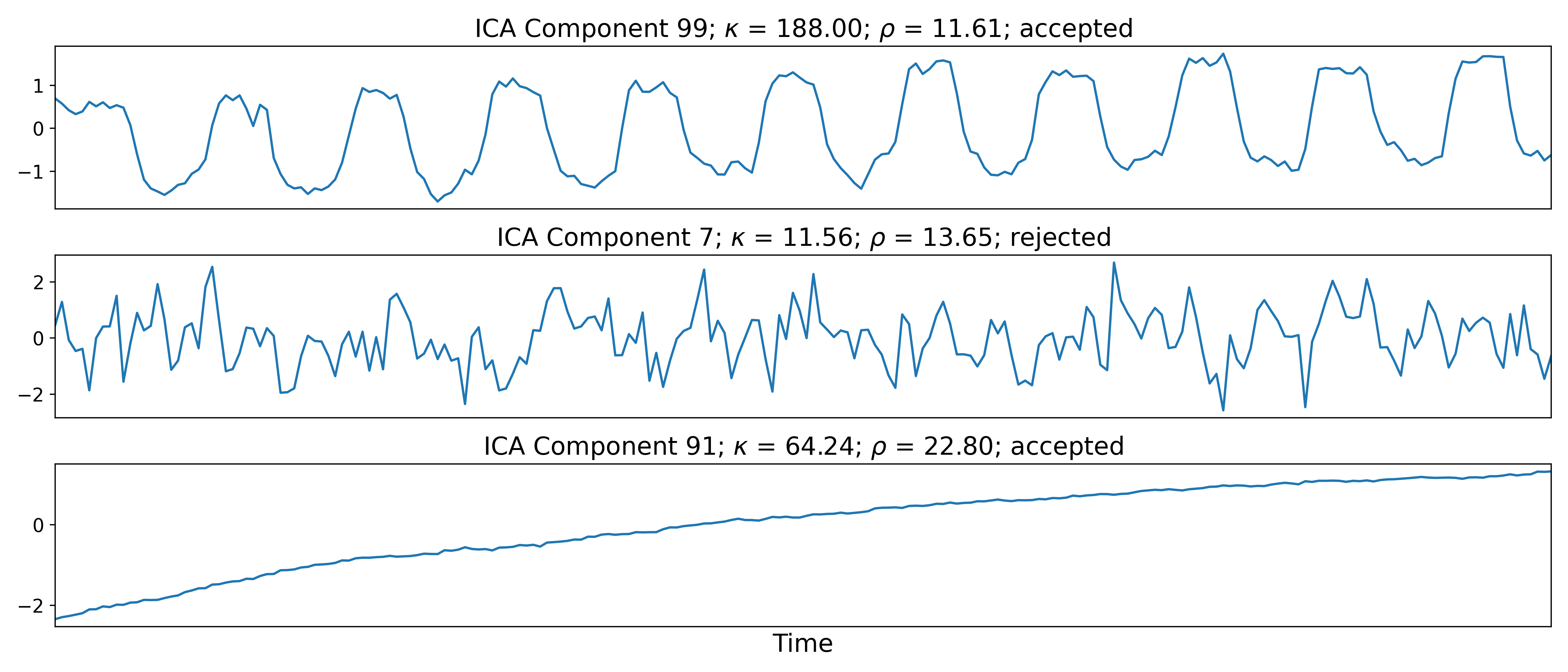
Next, tedana applies TE-dependent independent component analysis (ICA) in order to identify and remove TE-independent (i.e., non-BOLD noise) components. The dimensionally reduced optimally combined data are first subjected to ICA in order to fit a mixing matrix to the whitened data. This generates a number of independent timeseries (saved as desc-ICA_mixing.tsv), as well as parameter estimate maps which show the spatial loading of these components on the brain (desc-ICA_components.nii.gz).

_images/a13_ica_component_timeseries.png

Linear regression is used to fit the component time series to each voxel in each of the original, echo-specific data. This results in echo- and voxel-specific betas for each of the components. The beta values from the linear regression can be used to determine how the fluctuations (in each component timeseries) change across the echo times.

TE-dependence ( $R_2$ or $1/T_{2}^*$ ) and TE-independence ( $S_0$ ) models can then be fit to these betas. These models allow calculation of F-statistics for the $R_2$ and $S_0$ models (referred to as $\kappa$ and $\rho$ , respectively).

Tip

For more information on how TE-dependence and TE-independence models are estimated, see TE (In)Dependence Models.

The grey lines below shows how beta values (a.k.a. parameter estimates) change with echo time, for one voxel and one component. The blue and red lines show the predicted values for the $S_0$ and $T_2^*$ models, respectively, for the same voxel and component.

_images/a14_te_dependence_models_component_0.png

_images/a14_te_dependence_models_component_1.png

_images/a14_te_dependence_models_component_2.png

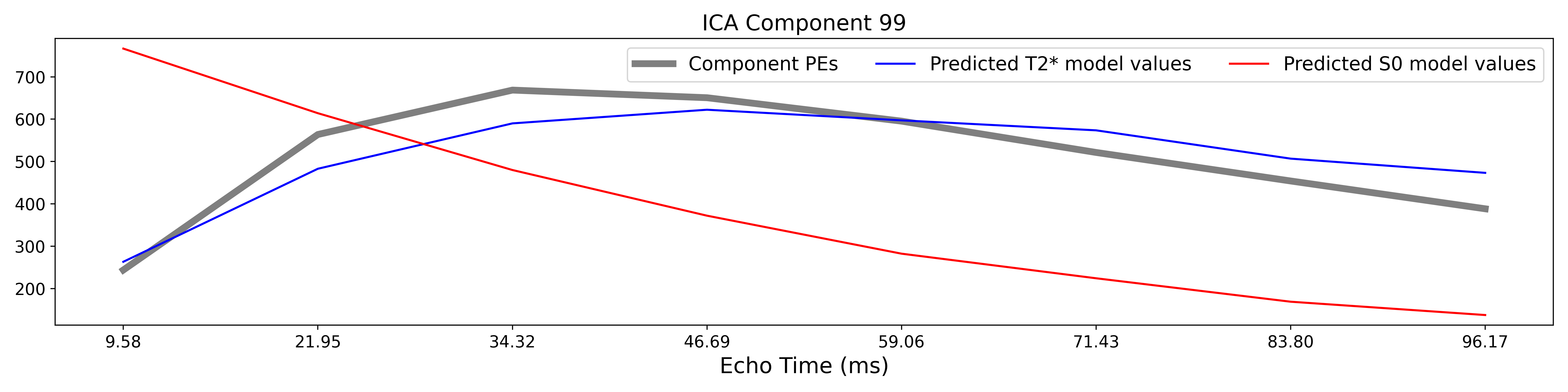
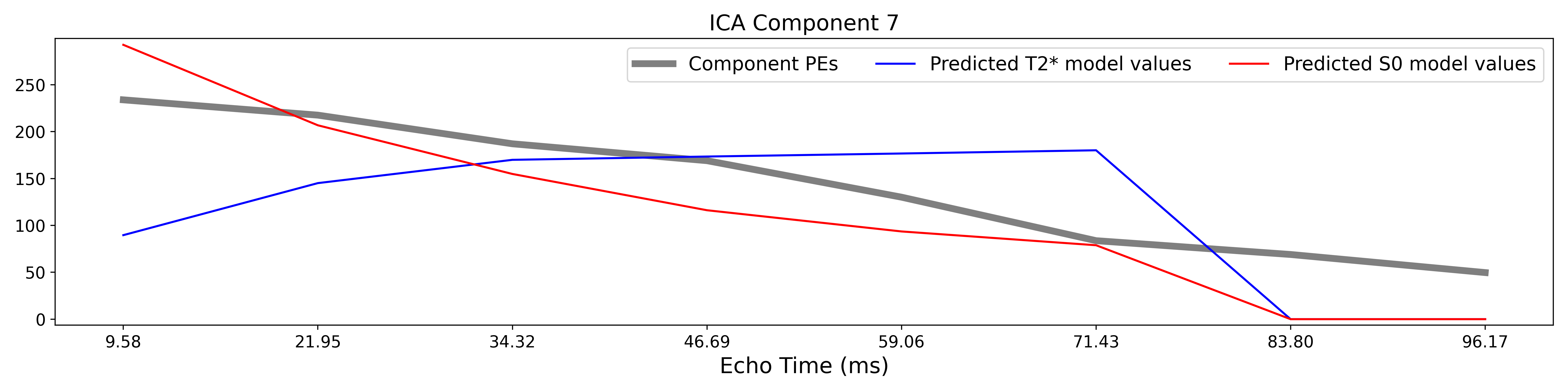
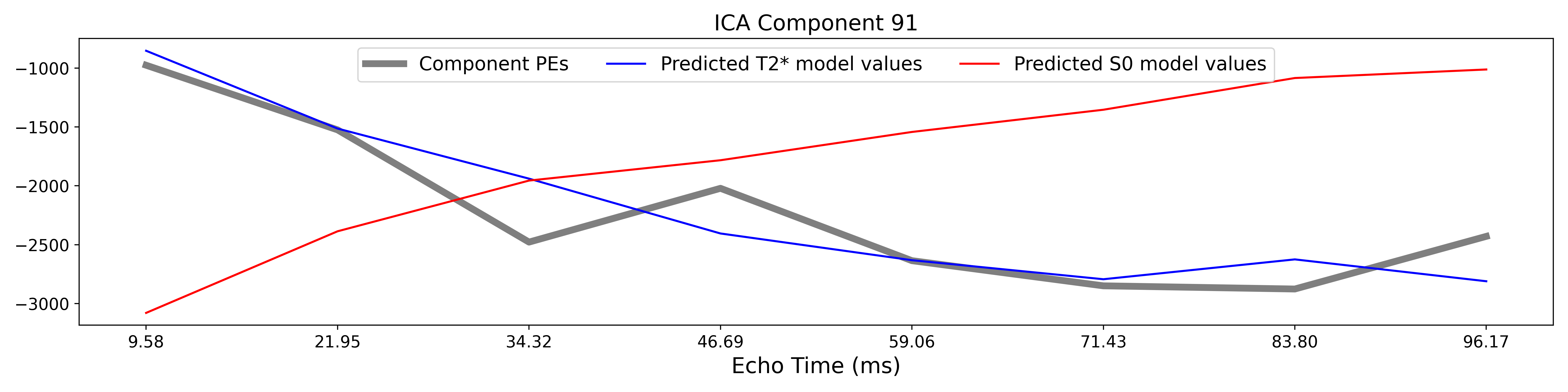
A decision tree is applied to $\kappa$ , $\rho$ , and other metrics in order to classify ICA components as TE-dependent (BOLD signal), TE-independent (non-BOLD noise), or neither (to be ignored). These classifications are saved in desc-tedana_metrics.tsv. The actual decision tree is dependent on the component selection algorithm employed. tedana includes two options kundu and minimal (which uses hardcoded thresholds applied to each of the metrics). These decision trees are detailed here.

Components that are classified as noise are projected out of the optimally combined data, yielding a denoised timeseries, which is saved as desc-optcomDenoised_bold.nii.gz.

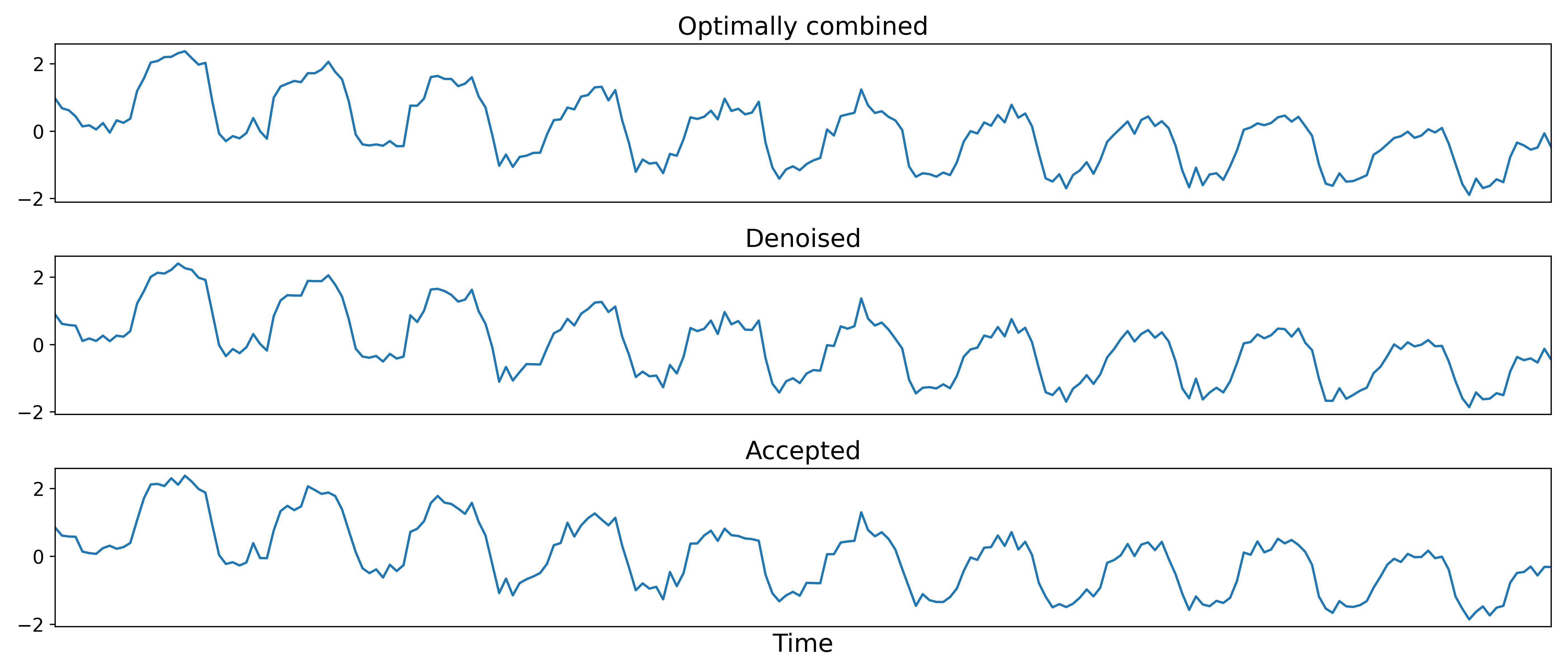
_images/a15_denoised_data_timeseries.png

Manual classification with RICA 

RICA is a tool for manual ICA classification. Once the .tsv file containing the result of manual component classification is obtained, it is necessary to re-run the tedana workflow passing the manual_classification.tsv file with the –ctab option. To save the output correctly, make sure that the output directory does not coincide with the input directory. See this example presented at MRITogether 2022 for a hands-on tutorial.

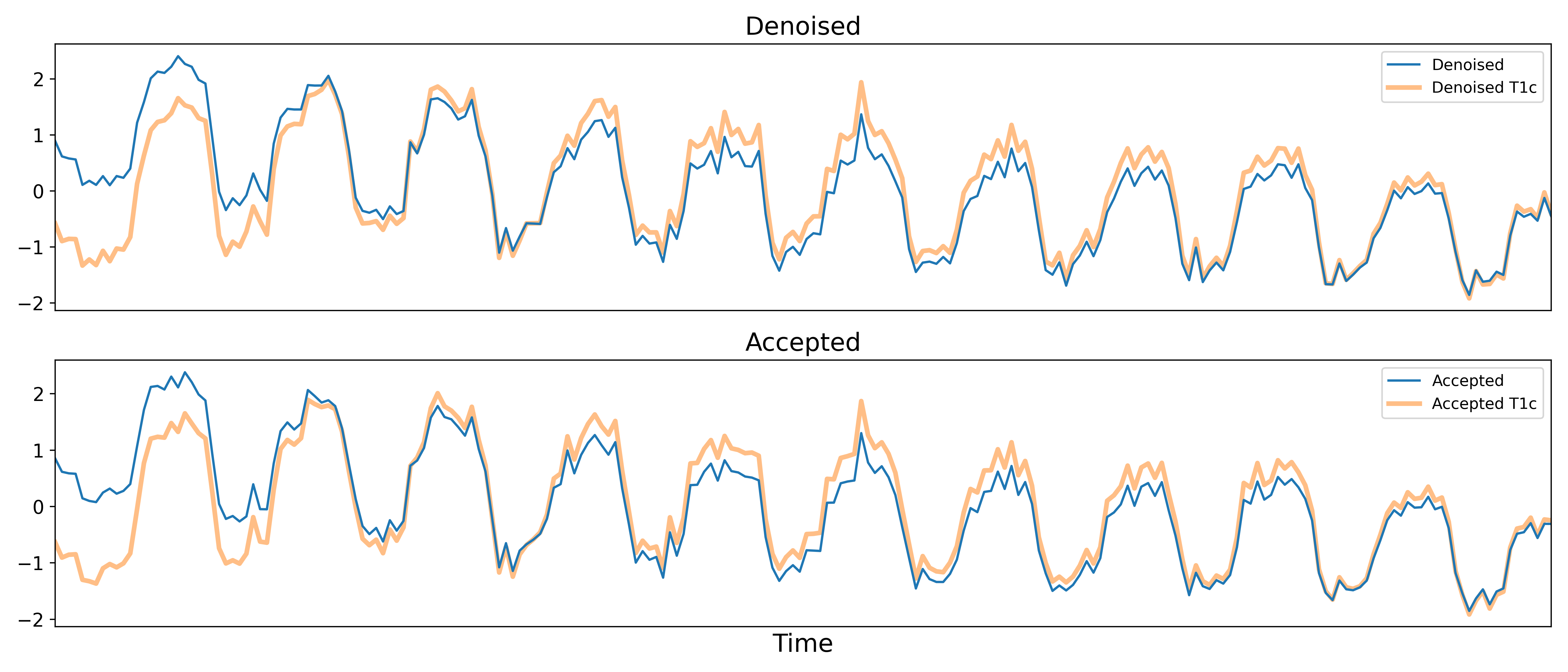
Removal of spatially diffuse noise (optional)

tedana.gscontrol.gscontrol_raw(), tedana.gscontrol.gscontrol_mmix()

Due to the constraints of ICA, TEDICA is able to identify and remove spatially localized noise components, but it cannot identify components that are spread out throughout the whole brain. See Power et al. (2018) for more information about this issue. One of several post-processing strategies may be applied to the ME-DN or ME-HK datasets in order to remove spatially diffuse (ostensibly respiration-related) noise. Methods which have been employed in the past include global signal regression (GSR), minimum image regression (MIR), anatomical CompCor, Go Decomposition (GODEC), and robust PCA. Currently, tedana implements GSR and MIR.