Outputs of tedana
When tedana is run, it outputs many files and an html report to help interpret the
results. This details the contents of all outputted files, explains the terminology
used for describing the outputs of classification, and details the contents of the html
report.
Output filename descriptions
The output include files for the optimally combined and denoised
data and many additional files to help understand the results and fascilitate
future processing. tedana allows for multiple file naming conventions. The key labels
and naming options for each convention that can be set using the --convention option
are in outputs.json. The output of tedana also includes a file called
registry.json or desc-tedana_registry.json that includes the keys and the matching
file names for the output. The table below lists both these keys and the default
“BIDS Derivatives” file names.
Standard filename outputs
Key: Filename |
Content |
|---|---|
“registry json”: desc-tedana_registry.json |
Mapping of file name keys to filename locations |
“data description json”: dataset_description.json |
Top-level metadata for the workflow. |
tedana_report.html |
The interactive HTML report. |
“combined img”: desc-optcom_bold.nii.gz |
Optimally combined time series. |
“denoised ts img”: desc-denoised_bold.nii.gz |
Denoised optimally combined time series. Recommended dataset for analysis. |
“adaptive mask img”: desc-adaptiveGoodSignal_mask.nii.gz |
Integer-valued mask used in the workflow, where each voxel’s value corresponds to the number of good echoes to be used for T2*/S0 estimation. Will be calculated whether original mask estimated within tedana or user-provided. All voxels with 1 good echo will be included in outputted time series but only voxels with at least 3 good echoes will be used in ICA and metric calculations |
“t2star img”: T2starmap.nii.gz |
Full estimated T2* 3D map. Values are in seconds. If a voxel has at least 1 good echo then the first two echoes will be used to estimate a value (an impresise weighting for optimal combination is better than fully excluding a voxel) |
“s0 img”: S0map.nii.gz |
Full S0 3D map. If a voxel has at least 1 good echo then the first two echoes will be used to estimate a value |
“PCA mixing tsv”: desc-PCA_mixing.tsv |
Mixing matrix (component time series) from PCA decomposition in a tab-delimited file. Each column is a different component, and the column name is the component number. |
“PCA decomposition json”: desc-PCA_decomposition.json |
Metadata for the PCA decomposition. |
“z-scored PCA components img”: desc-PCA_stat-z_components.nii.gz |
Component weight maps from PCA decomposition. Each map corresponds to the same component index in the mixing matrix and component table. Maps are in z-statistics. |
“PCA metrics tsv”: desc-PCA_metrics.tsv |
TEDPCA component table. A BIDS Derivatives-compatible TSV file with summary metrics and inclusion/exclusion information for each component from the PCA decomposition. |
“PCA metrics json”: desc-PCA_metrics.json |
Metadata about the metrics in |
“PCA cross component metrics json”: desc-PCACrossComponent_metrics.json |
Measures calculated across PCA compononents including
values for the full cost function curves for all
AIC, KIC, and MDL cost functions and the number of
components and variance explained for multiple options
Figures for the cost functions and variance explained
are also in
|
“ICA mixing tsv”: desc-ICA_mixing.tsv |
Mixing matrix (component time series) from ICA decomposition in a tab-delimited file. Each column is a different component, and the column name is the component number. |
“ICA components img”: desc-ICA_components.nii.gz |
Full ICA coefficient feature set. |
“z-scored ICA components img”: desc-ICA_stat-z_components.nii.gz |
Z-statistic component weight maps from ICA decomposition. Values are z-transformed standardized regression coefficients. Each map corresponds to the same component index in the mixing matrix and component table. |
“ICA decomposition json”: desc-ICA_decomposition.json |
Metadata for the ICA decomposition. |
“ICA metrics tsv”: desc-tedana_metrics.tsv |
TEDICA component table. A BIDS Derivatives-compatible TSV file with summary metrics and inclusion/exclusion information for each component from the ICA decomposition. |
“ICA metrics json”: desc-tedana_metrics.json |
Metadata about the metrics in
|
“ICA cross component metrics json”: desc-ICACrossComponent_metrics.json |
Metric names and values that are each a single number calculated across components. For example, kappa and rho elbows. |
“ICA decision tree json”: desc-ICA_decision_tree |
A copy of the inputted decision tree specification with an added “output” field for each node. The output field contains information about what happened during execution. |
“ICA status table tsv”: desc-ICA_status_table.tsv |
A table where each column lists the classification status of each component after each node was run. Columns are only added for runs where component statuses can change. |
“ICA accepted components img”: desc-ICAAccepted_components.nii.gz |
High-kappa ICA coefficient feature set |
“z-scored ICA accepted components img”: desc-ICAAcceptedZ_components.nii.gz |
Z-normalized spatial component maps |
report.txt |
A summary report for the workflow with relevant citations. |
“low kappa ts img”: desc-optcomRejected_bold.nii.gz |
Combined time series from rejected components. |
“high kappa ts img”: desc-optcomAccepted_bold.nii.gz |
High-kappa time series. This dataset does not include thermal noise or low variance components. Not the recommended dataset for analysis. |
“confounds tsv”: desc-confounds_timeseries.tsv |
Summary time series measures, including RMSE measures of T2*/S0 model fit. |
references.bib |
The BibTeX entries for references cited in report.txt. |
If verbose is set to True
Key: Filename |
Content |
|---|---|
“limited t2star img”: desc-limited_T2starmap.nii.gz |
Limited T2* map/time series. Values are in seconds. Unlike the full T2* maps, if only one 1 echo contains good data the limited map will have NaN |
“limited s0 img”: desc-limited_S0map.nii.gz |
Limited S0 map/time series. Unlike the full S0 maps, if only one 1 echo contains good data the limited map will have NaN |
“whitened img”: desc-optcom_whitened_bold |
The optimally combined data after whitening |
“echo weight [PCA|ICA] maps split img”: echo-[echo]_desc-[PCA|ICA]_components.nii.gz |
Echo-wise PCA/ICA component weight maps. |
“echo T2 [PCA|ICA] split img”: echo-[echo]_desc-[PCA|ICA]T2ModelPredictions_components.nii.gz |
Component- and voxel-wise R2-model predictions, separated by echo. |
“echo S0 [PCA|ICA] split img”: echo-[echo]_desc-[PCA|ICA]S0ModelPredictions_components.nii.gz |
Component- and voxel-wise S0-model predictions, separated by echo. |
“[PCA|ICA] component weights img”: desc-[PCA|ICA]AveragingWeights_components.nii.gz |
Component-wise averaging weights for metric calculation. |
“[PCA|ICA] component F-S0 img”: desc-[PCA|ICA]S0_stat-F_statmap.nii.gz |
F-statistic map for each component, for the S0 model. |
“[PCA|ICA] component F-T2 img”: desc-[PCA|ICA]T2_stat-F_statmap.nii.gz |
F-statistic map for each component, for the T2 model. |
“PCA reduced img”: desc-optcomPCAReduced_bold.nii.gz |
Optimally combined data after dimensionality reduction with PCA. This is the input to the ICA. |
“high kappa ts split img”: echo-[echo]_desc-Accepted_bold.nii.gz |
High-Kappa time series for echo number |
“low kappa ts split img”: echo-[echo]_desc-Rejected_bold.nii.gz |
Low-Kappa time series for echo number |
“denoised ts split img”: echo-[echo]_desc-Denoised_bold.nii.gz |
Denoised time series for echo number |
If fittype is “curvefit”
Key: Filename |
Content |
|---|---|
“t2star variance img”: stat-variance_desc-t2star_statmap.nii.gz |
Variance of the T2* estimates. |
“s0 variance img”: stat-variance_desc-s0_statmap.nii.gz |
Variance of the S0 estimates. |
“t2star-s0 covariance img”: stat-covariance_desc-t2star+s0_statmap.nii.gz |
Covariance of the T2* and S0 estimates. |
If tedort is True
Key: Filename |
Content |
|---|---|
“ICA orthogonalized mixing tsv”: desc-ICAOrth_mixing.tsv |
Mixing matrix with rejected components orthogonalized from accepted components |
If gscontrol includes ‘gsr’
Key: Filename |
Content |
|---|---|
“gs img”: desc-globalSignal_map.nii.gz |
Spatial global signal |
“confounds tsv”: desc-confounds_timeseries.tsv |
Time series of global signal from optimally combined data will be added to this file. |
“has gs combined img”: desc-optcomWithGlobalSignal_bold.nii.gz |
Optimally combined time series with global signal retained. |
“removed gs combined img”: desc-optcomNoGlobalSignal_bold.nii.gz |
Optimally combined time series with global signal removed. |
If gscontrol includes ‘mir’
(Minimal intensity regression, which may help remove some T1 noise and was an option in the MEICA v2.5 code, but never fully explained or evaluted in a publication)
Key: Filename |
Content |
|---|---|
“t1 like img”: desc-T1likeEffect_min.nii.gz |
T1-like effect |
“mir denoised img”: desc-optcomMIRDenoised_bold.nii.gz |
Denoised time series after MIR |
“ICA MIR mixing tsv”: desc-ICAMIRDenoised_mixing.tsv |
ICA mixing matrix after MIR |
“ICA accepted mir component weights img”: desc-ICAAcceptedMIRDenoised_components.nii.gz |
high-kappa components after MIR |
“ICA accepted mir denoised img”: desc-optcomAcceptedMIRDenoised_bold.nii.gz |
high-kappa time series after MIR |
Classification output descriptions
TEDPCA and TEDICA use component tables to track relevant metrics, component classifications, and rationales behind classifications. The component tables and additional information are stored as tsv and json files, labeled “ICA metrics” and “PCA metrics” in Standard filename outputs This section explains the classification codes those files in more detail. Understanding and building a component selection process covers the full process, and not just the descriptions of outputted files.
TEDPCA codes
In tedana PCA is used to reduce the number of dimensions (components) in the
dataset. Without this step, the number of components would be one less than
the number of volumes, many of those components would effectively be
Gaussian noise and ICA would not reliably converge. Standard methods for data
reduction use cost functions, like MDL, KIC, and AIC to estimate the variance
that is just noise and remove the lowest variance components under that
threshold.
By default, tedana uses AIC.
Of those three, AIC is the least agressive and will retain the most components.
Tedana includes additional kundu and kundu-stabilize approaches that
identify and remove components that don’t contain T2* or S0 signal and are more
likely to be noise. If the –tedpca kundu option is used, the PCA_metrics tsv
file will include an accepted vs rejected classification column and also a
rationale column of codes documenting why a PCA component removed. If MDL, KIC,
or AIC are used then the classification column will exist, but will include
include the accepted components and the rationale column will contain n/a”
When kundu is used, these are brief explanations of the the rationale codes
Code |
Classification |
Description |
|---|---|---|
P001 |
rejected |
Low Rho, Kappa, and variance explained |
P002 |
rejected |
Low variance explained |
P003 |
rejected |
Kappa equals fmax |
P004 |
rejected |
Rho equals fmax |
P005 |
rejected |
Cumulative variance explained above 95% (only in stabilized PCA decision tree) |
P006 |
rejected |
Kappa below fmin (only in stabilized PCA decision tree) |
P007 |
rejected |
Rho below fmin (only in stabilized PCA decision tree) |
ICA Classification Outputs
The component table is stored in desc-tedana_metrics.tsv or
tedana_metrics.tsv.
Each row is a component number.
Each column is a metric that is calculated for each component.
Short descriptions of each column metric are in the output log,
tedana_[date_time].tsv, and the actual metric calculations are in
collect.
The final two columns are classification and classification_tags.
classification should include accepted or rejected for every
component and rejected components are be removed through denoising.
classification_tags provide more information on why
components received a specific classification.
Each component can receive more than one tag.
The following tags are included depending if --tree is “minimal”, “meica”,
“tedana_orig” or if ica_reclassify is run. The same tags are included
for “meica” and “tedana_orig”
Tag |
Included in Tree |
Explanation |
|---|---|---|
Likely BOLD |
minimal,meica |
Accepted because likely to include some BOLD signal |
Unlikely BOLD |
minimal,meica |
Rejected because likely to include a lot of non-BOLD signal |
Low variance |
minimal,meica |
Accepted because too low variance to lose a degree-of-freedom by rejecting |
Less likely BOLD |
meica |
Rejected based on some edge criteria based on relative rankings of components |
Accept borderline |
meica |
Accepted based on some edge criteria based on relative rankings of components |
No provisional accept |
meica |
Accepted because because meica tree did not find any components to consider accepting so the conservative “failure” case is accept everything rather than rejecting everything |
manual reclassify |
manual_classify |
Classification based on user input. If done after automatic selection then the preceding tag from automatic selection is retained and this tag notes the classification was manually changed |
The decision tree is a list of nodes where the classification of each component could change. The information on which nodes and how classifications changed is in several places:
The information in the output log includes the name of each node and the count of components that changed classification during execution.
The same information is stored in the
ICA decision treejson file (see Output filename descriptions) in the “output” field for each node. That information is organized so that it can be used to generate a visual or text-based summary of what happened when the decision tree was run on a dataset.The
ICA status tablelists the classification status of each component after each node was run. This is particularly useful to trying to understand how a specific component ended receiving its classification.
ICA Components Report
The reporting page for the tedana decomposition presents a series of interactive plots designed to help you evaluate the quality of your analyses. This page describes the plots forming the reports as well as information on how to take advantage of the interactive functionalities. You can also play around with our demo.
Report Structure
The report is split into tabs, and only one tab is shown at a time. Select a tab to switch between them, or move between them with the left and right arrow keys.
Info: the command that was run, the system and library versions it was run with, a description of the workflow, and the references it cites.
ICA: the interactive component plots described below, the robust ICA clustering plot when
--ica_method robusticawas used, and the external regressor correlations when external regressors were provided.Tree: the component selection decision tree and the classification of every component at each node of that tree.
Carpet: the carpet plots, and the global signal removal plots when
--gscontrolwas used.Decay: organized into three sections — Masking (the adaptive mask), Parameter estimates (the T2* and S0 maps and histograms), and Curve-fit quality (the RMSE map and time series, the T2*/S0 estimate variance and covariance maps).
The Decay and Tree tabs are only shown when a workflow produces their contents.
For example, ica_reclassify does not re-estimate T2* and S0, so a report
written to a new output directory by that workflow has no Decay tab.
The image below shows a representative report. The left is a summary view which contains information on all components and the right presents additional information for an individual component. One can hover over any pie chart wedge or data point in the summary view to see additional information about a component. Clicking on a component will select the component and the additional information will appear to the right. The left and right arrow keys cycle through compononents in the order they appear on the pie chart.
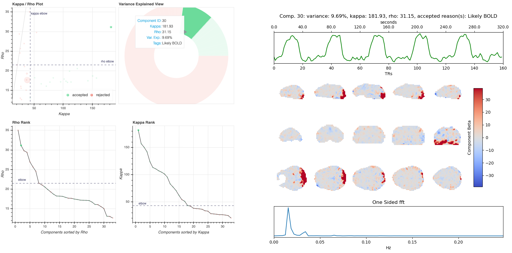
Summary View
This view provides an overview of the decomposition and component selection results. It includes four different plots.
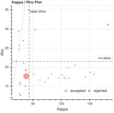
Kappa/Rho Scatter: This is a scatter plot of Kappa vs. Rho features for all components. In the plot, each dot represents a different component. The x-axis represents the kappa feature, and the y-axis represents the rho feature. Kappa is a summary metric for how much BOLD information might be in a component and rho is a summary metric for how much non-BOLD information is in a component. Thus a component with a higher kappa and lower rho value is more likely to be retained. The solid gray line is
 . Color is used to label accepted (green) or rejected (red)
components. The size of the circle is the amount of variance explained by the
component so larger circle (higher variance) that seems misclassified is worth
closer inspection. The component classification process uses kappa and rho elbow
thresholds (black dashed lines) along with other criteria. Most accepted
components should be greater than the kappa elbow and less than the rho elbow.
Accepted or rejected components that don’t cross those thresholds might be
worth additional inspection. Hovering over a component also shows a Tag
that explains why a component received its classification.
. Color is used to label accepted (green) or rejected (red)
components. The size of the circle is the amount of variance explained by the
component so larger circle (higher variance) that seems misclassified is worth
closer inspection. The component classification process uses kappa and rho elbow
thresholds (black dashed lines) along with other criteria. Most accepted
components should be greater than the kappa elbow and less than the rho elbow.
Accepted or rejected components that don’t cross those thresholds might be
worth additional inspection. Hovering over a component also shows a Tag
that explains why a component received its classification.
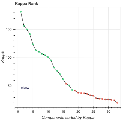
Kappa Scree Plot: This scree plot provides a view of the components ranked by Kappa. As in the previous plot, each dot represents a component. The color of the dot informs us about classification status. The dashed line is the kappa elbow threshold. In this plot, size is not related to variance explained, but you can see the variance explained by hovering over any dot.
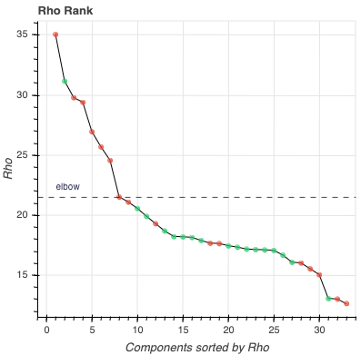
Rho Scree Plot: This scree plot provides a view of the components ranked by Rho. As in the previous plot, each dot represents a component. The color of the dot informs us about classification status. The dashed line is the rho elbow threshold. Size is not related to variance explained.
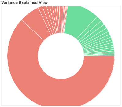
Variance Explained Plot: This pie plot provides a summary of how much variance is explained by each individual component. In this plot, each component is represented as a wedge, whose size is directly related to the amount of variance explained. The color of the wedge is the classification status of the component. For this view, components are sorted by classification first, and inside each classification group by variance explained. The center of the plot shows the total number of components, the number of components that are accepted or rejected, and the relative variance explained by all the accepted or rejected components.
Individual Component View
This view provides detailed information about an individual component (selected in the summary view, see below). It includes three different plots.
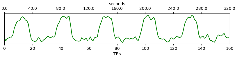
Time series: This plot shows the time series associated with a given component (selected in the summary view). The x-axis represents time (in units of TR and seconds), and the y-axis represents signal levels (in arbitrary units). Finally, the color of the trace informs us about the component classification status. Plausibly BOLD-weighted components might have responses that follow the task design, while components that are less likely to be BOLD-weighted might have large signal spikes or slow drifts. If a high variance component time series initially has a few very high magnitude volumes, that is a sign non-steady state volumes were not removed before running
tedana. Keeping these volumes might results in a suboptimal ICA results.tedanashould be run without any initial non-steady state volumes. The title of this plot shows the component number, the classification status, the rationale tags, the variance explained by the component, and the kappa and rho values.
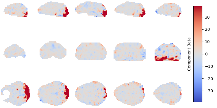
Component beta map: This plot shows the map of the relative beta coefficients associated with a given component (selected in the summary view). If one wants to look at these maps in more detail, they can be found in the
z-scored ICA components imgfile (see Output filename descriptions). The same weights could be flipped postive/negative so relative values are more relevant that what is very positive vs negative. Plausibly BOLD-weighted components should have larger hotspots in area that follow cortical or cerebellar brain structure. Hotspots in ventricles, on the edges of the brain or slice-specific or slice-alternating effects are signs of artifacts.
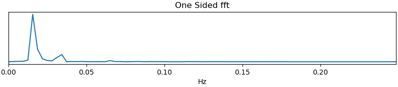
Spectrum: This plot shows the spectrogram associated with a given component (selected in the summary view). The x-axis represents frequency (in Hz), and the y-axis represents spectral amplitude. BOLD-weighted signals will likely have most power below 0.1Hz. Peaks at higher frequencies are signs of non-BOLD signals. A respiration artifact might be around 0.25-0.33Hz and a cardiac artifact might be around 1Hz. This plot shows the maximum resolvable frequency given the TR, so those higher frequencies might fold over to different peaks that are still above 0.1Hz. Respirator and cardiac fluctuation artifacts are also sometimes visible in the time series.
Reports User Interactions
As previously mentioned, all summary plots in the report allow user interactions. While the Kappa/Rho Scatter plot allows full user interaction (see the toolbar that accompanies the plot and the example below), the other three plots allow the user to select components and update the figures.

The table below includes information about all available interactions
Interaction |
Icon |
Description |
|---|---|---|
Pan |
|
Allows the user to pan a plot by left-dragging a mouse across the plot region. |
Wheel Zoom |
|
Zoom the plot in and out, centered on the current mouse location. |
Box Zoom |
|
Define a rectangular region of a plot to zoom to by dragging the mouse over the plot region. |
Tap |
|
Select a component by clicking a dot or wedge. Once a component is selected, the plots forming the individual component view update to show component specific information. |
Save |
|
Saves an image reproduction of the plot in PNG format. |
Reset |
|
Resets the data bounds of the plot to their values when the plot was initially created. |
Hover |
|
If active, the plot displays informational tooltips whenever the cursor is directly over a plot element. |
Crosshair |
|
Draws a crosshair annotation over the plot, centered on the current mouse position |


Note
Specific user interactions can be switched on/off by clicking on their associated icon within the toolbar of a given plot. Active interactions show an horizontal blue line underneath their icon, while inactive ones lack the line.
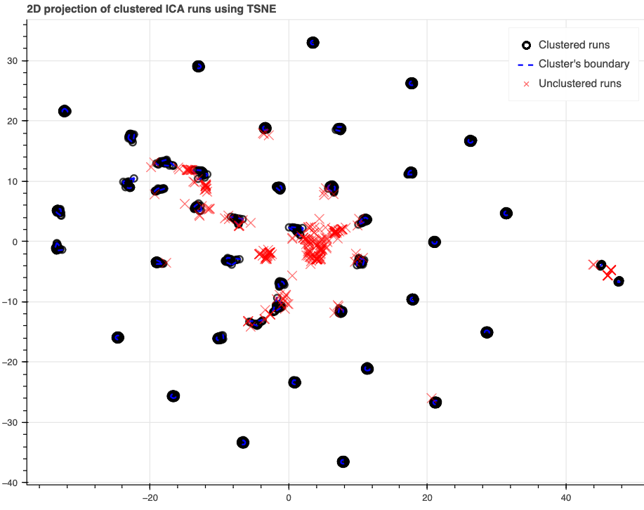
RobustICA Component Clusters
This plot will appear when the --ica_method robustica option is used.
RobustICA runs multiple iterations of ICA and identifies stable components
across iterations. This plot uses t-SNE to plot the components in 2D.
Each marker is a component from one iteration.
Components that are in stable clusters are black dots
and the dashed blue line surrounds the cluster.
Hover text shows the cluster number for each dot.
Components that are not in stable clusters are red x’s.
This figure is a work-in-progress in attempting to find ways to evaluate
robustICA results.
In general, tight clusters of black dots are better.
When evaluating results, a run with more diffuse clusters than others
with the same acquisition parameters,
but it’s unclear what variations are genuinely problemmatic.
The red x’s sometimes appear in clusters that are below the threshold
for being a cluster, but it’s unclear how to decide if clusters were missed.
If a cluster has some black dots that are far from others in the cluster,
that might be an effect of the t-SNE dimensionality reduction.
The goal of future work will be to improve visualizations
and quantification of clusters.
Decision Tree
The Tree tab summarizes how the component selection decision tree classified the components, using two tables.
The first table lists every node of the decision tree in the order it was applied.
For each node it shows the function that was run, a short label describing what the
node did, and the number of components that did and did not meet the node’s condition.
The last two counts are only reported for nodes that make a decision, so they are
blank for setup nodes. This table is a flat view of the same information stored in
desc-ICA_decision_tree.json, and is a quick way to see which criteria drove the
classification and how many components each one affected.
The second table shows the classification of every component after each node of the
tree, with one row per component and one column per node. Reading across a row shows
how a component’s label evolved, for example from unclassified to rejected,
as the tree was applied. It is the same information stored in
desc-ICA_status_table.tsv, and is useful for understanding why a specific
component ended up accepted or rejected. The table can be scrolled horizontally when
a run has many nodes.
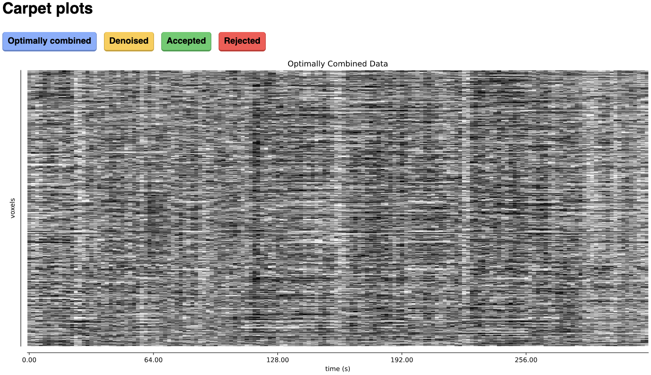
Carpet plots
The Carpet tab of tedana’s interactive reports includes carpet plots for the main outputs of the workflow:
the optimally combined data, the denoised data, the high-Kappa (accepted) data, and the low-Kappa (rejected) data. Each row is a voxel
and the grayscale is the relative signal changes across time. After denoising, voxels that look very different from others across time
or time points that are uniformly high or low across voxels are concerning. These carpet plots can be help as a quick quality check for
data, but since some neural signals really are more global than others and there are voxelwise differences in responses, quality checks
should not overly focus on carpet plots and should examine these results in context with other quality measures.
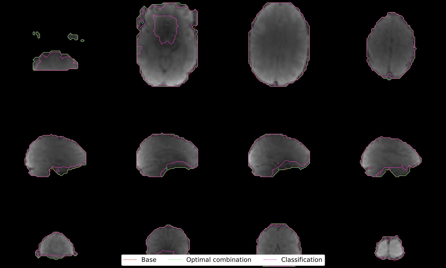
Adaptive Mask Summary Plot
The Decay tab opens with a summary plot of the adaptive mask.
This figure overlays contours reflecting the boundaries of the following masks onto the mean optimally combined data:
Initial mask only: The initla mask, either provided by the user or generated automatically using
compute_epi_mask.Optimal combination: The mask used for optimal combination and denoising. This corresponds to values greater than or equal to 1 (at least 1 good echo) in the adaptive mask.
Classification: The mask used for the decomposition and component classification steps. This corresponds to values greather than or equal to 3 (at least 3 good echoes) in the adaptive mask. Both the denoised and optimally combined outputs will include all voxels in the “optimal combination” mask, but only voxels in the “classification” mask will be included in the ICA decomposition and component classification steps.
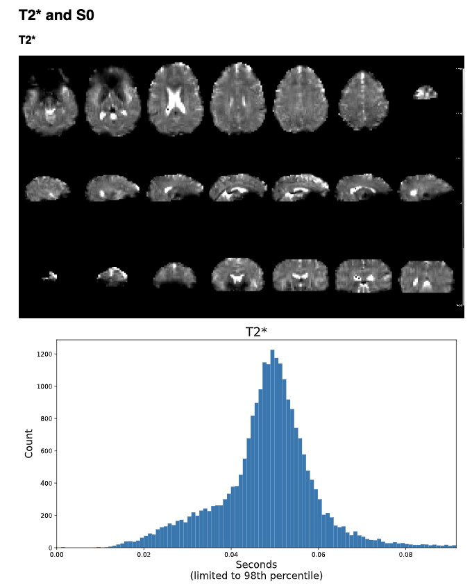
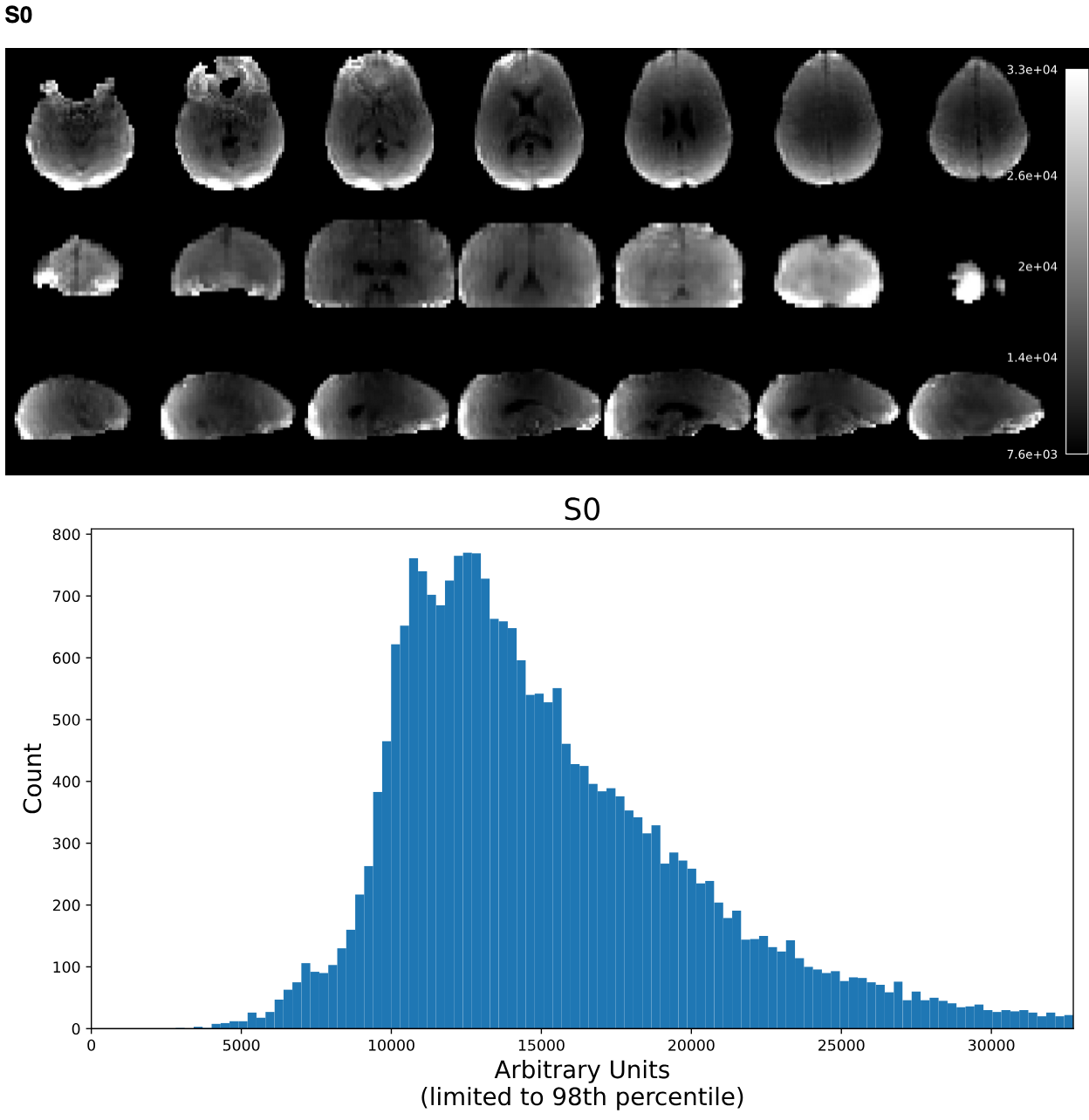
T2* and S0 Summary Plots
Below the adaptive mask plot, in the same Decay tab, are summary plots for the T2* and S0 maps. Each map has two figures: a spatial map of the values and a histogram of the voxelwise values. The T2* map should look similar to T2 maps and be brightest in the ventricles and darkest in areas of largest susceptibility. The S0 map should roughly follow the signal-to-noise ratio and will be brightest near the surface near RF coils.
It is important to note that the histogram is limited from 0 to the 98th percentile of the data to improve readability.
Decay Model Fit Plots
Below the T2* and S0 summary plots, in the same Decay tab, are the decay model fit plots. These plots show residual mean squared error (RMSE) values for the monoexponential decay model, based on the T2* and S0 maps.
The first plot is the mean RMSE brain plot, which shows the mean RMSE over time for each voxel in the brain. This plot is limited from the 2nd percentile to the 98th percentile.
The second plot is a time series of RMSE values across the brain, over time. This plot includes the median RMSE time series, along with an error band representing the 25th and 75th percentiles, and dotted lines indicating the 2nd and 98th percentile RMSE values.
The fit quality will vary depending on acquisition parameters and will likely be worse near signal drop-out areas. For a study with consistent acquisition parameters, relatively high RMSE values for runs or timepoints might be a marker of an underlying data quality issue.

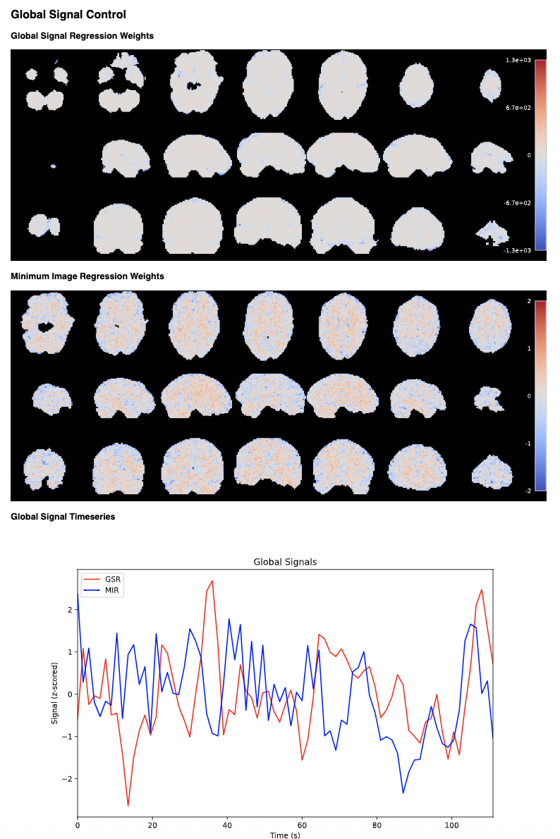
Global Signal Removal Plots
The Carpet tab also shows the global signal removal plots, if --gscontrol was used.
These plots show the voxel-wise global signal weights and the global signal time series.
Rica Interactive Reports
In addition to the standard HTML report, tedana generates a launcher script for
Rica, an interactive web-based visualization
tool for exploring ICA components. Rica provides a more detailed and interactive
way to inspect individual components, including 3D brain visualization using NiiVue.
The Rica Launcher Script
Every tedana run creates a launcher script open_rica_report.py in the output
directory. When you run this script, it will:
Check for Rica files (from environment variable, cache, or download)
Download Rica from the ME-ICA/rica GitHub releases if not already available (cached locally for future use)
Copy Rica files to
output/rica/Start a local HTTP server
Open Rica in your default web browser
This approach keeps tedana execution fast (no network calls during analysis)
while providing easy access to Rica visualization on demand.
Opening Rica
After running tedana, open the Rica visualization:
cd output
python open_rica_report.py
Press Ctrl+C in the terminal to stop the server when you’re done.
Rica Output Files
The following files are created in the output directory:
File |
Description |
|---|---|
|
Cross-platform launcher script (created by tedana) |
|
Rica web application (created when launcher is run) |
|
HTTP server script (created when launcher is run) |
Note
The rica/ directory is created when you run open_rica_report.py, not
during the tedana analysis. This keeps tedana fast and network-independent.
Platform Support
Rica reports work on all major platforms:
Linux: Cache stored in
~/.cache/tedana/ricamacOS: Cache stored in
~/Library/Caches/tedana/ricaWindows: Cache stored in
%LOCALAPPDATA%/tedana/rica
The launcher script automatically finds an available port if the default (8000) is busy.
Note
Rica requires an internet connection for the initial download when you first run
open_rica_report.py. Once cached, Rica can be used offline.
Using a Local Rica Bundle (Advanced)
For advanced users and developers who need to use a custom Rica build or work offline,
you can point the launcher script to a local Rica installation using the TEDANA_RICA_PATH
environment variable.
The path should point to a directory containing the required Rica files:
index.html- The Rica web applicationrica_server.py- HTTP server with CORS support
Setting the environment variable:
# Set for current session
export TEDANA_RICA_PATH=/path/to/rica/build

# Then run the launcher script
python open_rica_report.py
To make this permanent, add the export line to your shell configuration file
(e.g., ~/.bashrc, ~/.zshrc, or ~/.bash_profile).
Note
If TEDANA_RICA_PATH is not set, the launcher script will automatically download
Rica from GitHub and cache it locally.
For Rica developers:
If you are developing Rica and have a local build, you can point the launcher to your build output directory:
# Build Rica locally
cd ~/GitHub/rica
npm run build

# Set the environment variable to use the local build
export TEDANA_RICA_PATH=~/GitHub/rica/build

# Run the launcher script
python open_rica_report.py
Troubleshooting Rica
Rica download fails:
If Rica fails to download from GitHub when running open_rica_report.py,
you may see an error like:
Failed to download Rica: <urlopen error ...>
Possible solutions:
Check your internet connection - Ensure you can access GitHub.
Use a local Rica bundle - Download Rica manually and set
TEDANA_RICA_PATH:# Download Rica release manually wget https://github.com/ME-ICA/rica/releases/latest/download/index.html wget https://github.com/ME-ICA/rica/releases/latest/download/rica_server.py # Place files in a directory and set the environment variable mkdir ~/rica-bundle mv index.html rica_server.py ~/rica-bundle/ export TEDANA_RICA_PATH=~/rica-bundle # Run the launcher python open_rica_report.py
Use the standard HTML report - The standard HTML report in the output directory provides similar functionality without requiring Rica.
Force re-downloading Rica:
To force a fresh download of Rica (e.g., to get a newer version):
python open_rica_report.py --force-download
Clearing the Rica cache:
If Rica files become corrupted and you want to clear the cache:
# Linux
rm -rf ~/.cache/tedana/rica

# macOS
rm -rf ~/Library/Caches/tedana/rica

# Windows (PowerShell)
Remove-Item -Recurse -Force "$env:LOCALAPPDATA\tedana\rica"
The next time you run open_rica_report.py, Rica will be re-downloaded.
Port conflicts:
When opening Rica, if port 8000 is already in use, the launcher script automatically tries the next available port (8001, 8002, etc.). If you see:
Error: Could not find free port starting from 8000
This means ports 8000-8009 are all in use. You can specify a different starting port:
python open_rica_report.py --port 9000
Browser does not open automatically:
If the browser doesn’t open, you can:
Open the URL manually (displayed in the terminal output)
Use the
--no-openflag and open the URL yourself:python open_rica_report.py --no-open # Then open http://localhost:8000/rica/index.html in your browser
Browser shows old version of Rica after update:
See the Rica troubleshooting guide for solutions to browser caching issues.
Citable workflow summaries
tedana generates a report for the workflow, customized based on the parameters used and including relevant citations.
The report is saved in a plain-text file, report.txt, in the output directory.
An example report
Note
The boilerplate text includes citations in LaTeX format. \citep refers to parenthetical citations, while \cite refers to textual ones.
TE-dependence analysis was performed on input data using the tedana workflow \citep{dupre2021te}. An adaptive mask was then generated, in which each voxel’s value reflects the number of echoes with ‘good’ data. A two-stage masking procedure was applied, in which a liberal mask (including voxels with good data in at least the first echo) was used for optimal combination, T2*/S0 estimation, and denoising, while a more conservative mask (restricted to voxels with good data in at least the first three echoes) was used for the component classification procedure. Multi-echo data were then optimally combined using the T2* combination method \citep{posse1999enhancement}. Next, components were manually classified as BOLD (TE-dependent), non-BOLD (TE-independent), or uncertain (low-variance). This workflow used numpy \citep{van2011numpy}, scipy \citep{virtanen2020scipy}, pandas \citep{mckinney2010data,reback2020pandas}, scikit-learn \citep{pedregosa2011scikit}, nilearn, bokeh \citep{bokehmanual}, matplotlib \citep{Hunter2007}, and nibabel \citep{brett_matthew_2019_3233118}. This workflow also used the Dice similarity index \citep{dice1945measures,sorensen1948method}.
References
Note
The references are also provided in the
references.biboutput file.@Manual{bokehmanual, title = {Bokeh: Python library for interactive visualization}, author = {{Bokeh Development Team}}, year = {2018}, url = {https://bokeh.pydata.org/en/latest/}, } @article{dice1945measures, title={Measures of the amount of ecologic association between species}, author={Dice, Lee R}, journal={Ecology}, volume={26}, number={3}, pages={297--302}, year={1945}, publisher={JSTOR}, url={https://doi.org/10.2307/1932409}, doi={10.2307/1932409} } @article{dupre2021te, title={TE-dependent analysis of multi-echo fMRI with* tedana}, author={DuPre, Elizabeth and Salo, Taylor and Ahmed, Zaki and Bandettini, Peter A and Bottenhorn, Katherine L and Caballero-Gaudes, C{\'e}sar and Dowdle, Logan T and Gonzalez-Castillo, Javier and Heunis, Stephan and Kundu, Prantik and others}, journal={Journal of Open Source Software}, volume={6}, number={66}, pages={3669}, year={2021}, url={https://doi.org/10.21105/joss.03669}, doi={10.21105/joss.03669} } @inproceedings{mckinney2010data, title={Data structures for statistical computing in python}, author={McKinney, Wes and others}, booktitle={Proceedings of the 9th Python in Science Conference}, volume={445}, number={1}, pages={51--56}, year={2010}, organization={Austin, TX}, url={https://doi.org/10.25080/Majora-92bf1922-00a}, doi={10.25080/Majora-92bf1922-00a} } @article{pedregosa2011scikit, title={Scikit-learn: Machine learning in Python}, author={Pedregosa, Fabian and Varoquaux, Ga{\"e}l and Gramfort, Alexandre and Michel, Vincent and Thirion, Bertrand and Grisel, Olivier and Blondel, Mathieu and Prettenhofer, Peter and Weiss, Ron and Dubourg, Vincent and others}, journal={the Journal of machine Learning research}, volume={12}, pages={2825--2830}, year={2011}, publisher={JMLR. org}, url={http://jmlr.org/papers/v12/pedregosa11a.html} } @article{posse1999enhancement, title={Enhancement of BOLD-contrast sensitivity by single-shot multi-echo functional MR imaging}, author={Posse, Stefan and Wiese, Stefan and Gembris, Daniel and Mathiak, Klaus and Kessler, Christoph and Grosse-Ruyken, Maria-Liisa and Elghahwagi, Barbara and Richards, Todd and Dager, Stephen R and Kiselev, Valerij G}, journal={Magnetic Resonance in Medicine: An Official Journal of the International Society for Magnetic Resonance in Medicine}, volume={42}, number={1}, pages={87--97}, year={1999}, publisher={Wiley Online Library}, url={https://doi.org/10.1002/(SICI)1522-2594(199907)42:1<87::AID-MRM13>3.0.CO;2-O}, doi={10.1002/(SICI)1522-2594(199907)42:1<87::AID-MRM13>3.0.CO;2-O} } @software{reback2020pandas, author = {The pandas development team}, title = {pandas-dev/pandas: Pandas}, month = feb, year = 2020, publisher = {Zenodo}, version = {latest}, doi = {10.5281/zenodo.3509134}, url = {https://doi.org/10.5281/zenodo.3509134} } @article{sorensen1948method, title={A method of establishing groups of equal amplitude in plant sociology based on similarity of species content and its application to analyses of the vegetation on Danish commons}, author={Sorensen, Th A}, journal={Biol. Skar.}, volume={5}, pages={1--34}, year={1948} } @article{van2011numpy, title={The NumPy array: a structure for efficient numerical computation}, author={Van Der Walt, Stefan and Colbert, S Chris and Varoquaux, Gael}, journal={Computing in science \& engineering}, volume={13}, number={2}, pages={22--30}, year={2011}, publisher={IEEE}, url={https://doi.org/10.1109/MCSE.2011.37}, doi={10.1109/MCSE.2011.37} } @article{virtanen2020scipy, title={SciPy 1.0: fundamental algorithms for scientific computing in Python}, author={Virtanen, Pauli and Gommers, Ralf and Oliphant, Travis E and Haberland, Matt and Reddy, Tyler and Cournapeau, David and Burovski, Evgeni and Peterson, Pearu and Weckesser, Warren and Bright, Jonathan and others}, journal={Nature methods}, volume={17}, number={3}, pages={261--272}, year={2020}, publisher={Nature Publishing Group}, url={https://doi.org/10.1038/s41592-019-0686-2}, doi={10.1038/s41592-019-0686-2} }