TE (In)Dependence Models
Functional MRI signal can be described in terms of fluctuations in  and
and  .
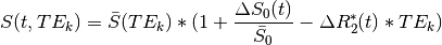
In the below equation,
.
In the below equation,  is signal at a given time
  and for a given echo time
  .
.
 is the mean signal across time for the echo time
.
is the mean signal across time for the echo time
.
 is the difference in at time
from the average (
is the difference in at time
from the average ( ).
).
 is the difference in
  at time
from the average .
at time
from the average .
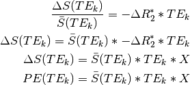
If we ignore time, this can be simplified to
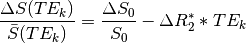
In order to evaluate whether signal change is being driven by fluctuations in
either or , one can break this overall model
into submodels by zeroing out certain terms.
For a TE-independence model, if there were no fluctuations in :
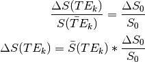
Note that TE is not a parameter in this model. Hence, this model is TE-independent.
Also,  is a scalar (i.e., doesn’t change with
TE), so we can just ignore that, which means we only use
is a scalar (i.e., doesn’t change with
TE), so we can just ignore that, which means we only use  (mean echo-wise signal).
Thus, the model becomes  , where we
fit X to the data using regression and evaluate model fit.
, where we
fit X to the data using regression and evaluate model fit.
For TEDPCA/TEDICA, we use regression to get parameter estimates (PEs; not beta
values) for component time-series against echo-specific data, and substitute
those PEs for .
Thus, to assess the TE-independence of a component, we use the model
 , fit X to the data, and evaluate model
fit.
, fit X to the data, and evaluate model
fit.
For a TE-dependence model, if there were no fluctuations in :
Note that TE is a parameter in this model. Hence, it is TE-dependent.
As an example, let us simulate some data. We will simulate signal decay for two time points, as well as the signal decay for the hypothetical overall average over time. In one time point, only S0 will fluctuate. In the other, only R2* will fluctuate.
Note
To make things easier, we’re simulating these data with echo times of 0 to 200 milliseconds, at 1ms intervals. In real life, you’ll generally only have 3-5 echoes to work with. Real signal from each echo will be contaminated with random noise and will have influences from both S0 and R2*.
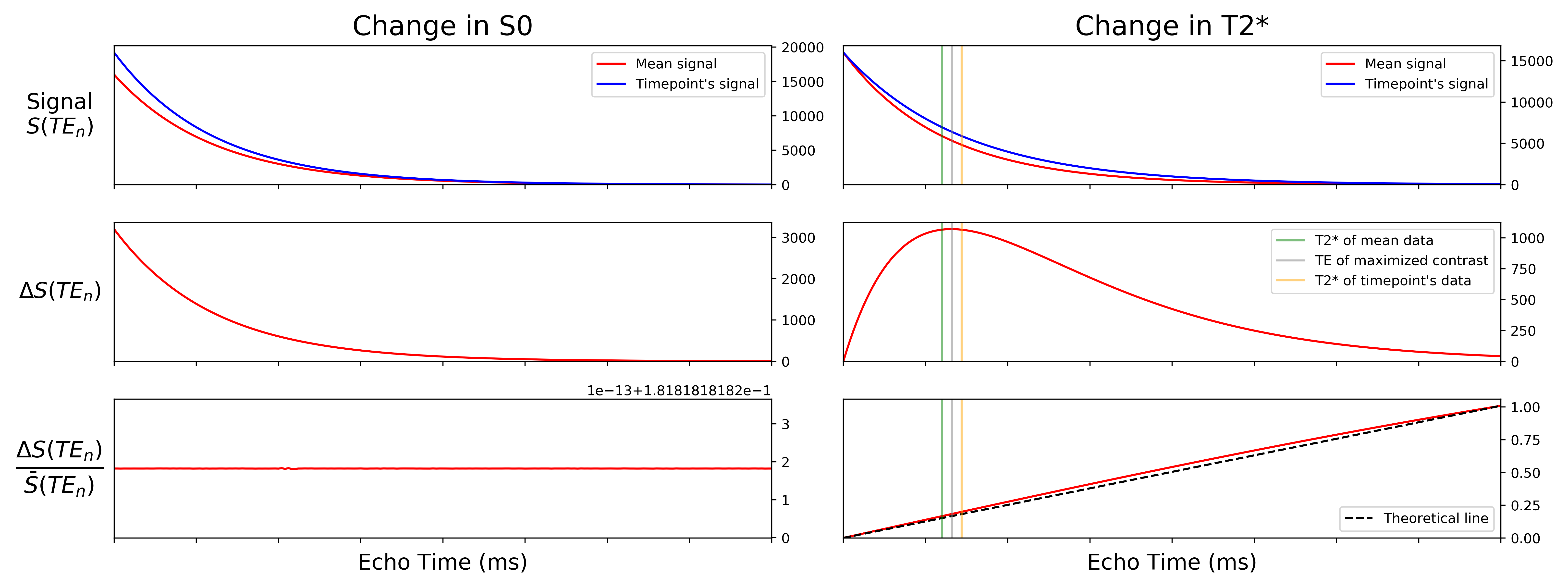
We can see that  has very different curves for the two
simulated datasets.
Moreover, as expected,
has very different curves for the two
simulated datasets.
Moreover, as expected,  is flat
across echoes for the S0-fluctuating data and scales roughly linearly with TE
for the R2*-fluctuating data.
is flat
across echoes for the S0-fluctuating data and scales roughly linearly with TE
for the R2*-fluctuating data.
We then fit our TE-dependence and TE-independence models to the
data, which gives us predicted data for each model for
each dataset.
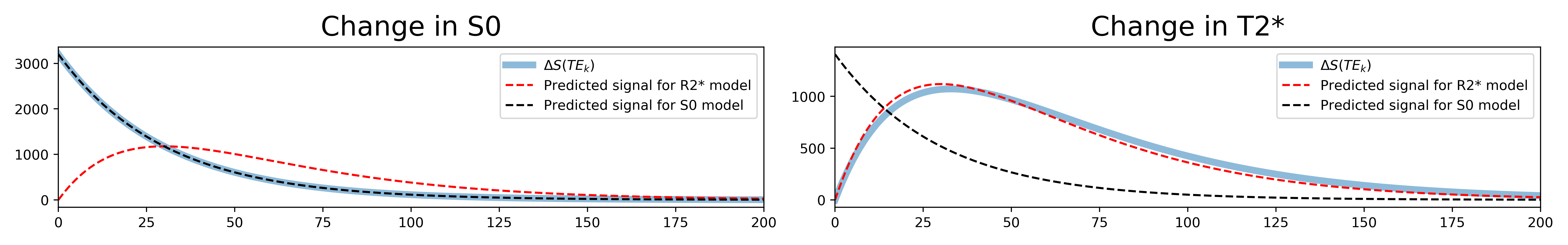
As expected, the S0 model fits perfectly to the S0-fluctuating dataset, while the R2* model fits quite well to the R2*-fluctuating dataset.
The actual model fits can be calculated as F-statistics. Then, the F-statistics per voxel are averaged across voxels into the Kappa and Rho pseudo-F-statistics.
Now let us see how this extends to time series, components, and component parameter estimates.
We have the means to simulate T2*- and S0-based fluctuations, so here we have compiled two component time series- one T2*-based and one S0-based. Both time series share the same level of percent signal change (a standard deviation equivalent to 5% of the mean), although the mean S0 (16000) is very different from the mean T2* (30). We can then average those two components with different weights to create components that are T2*- or S0-based to various degrees. In this case, both T2* and S0 contribute equally to the component.
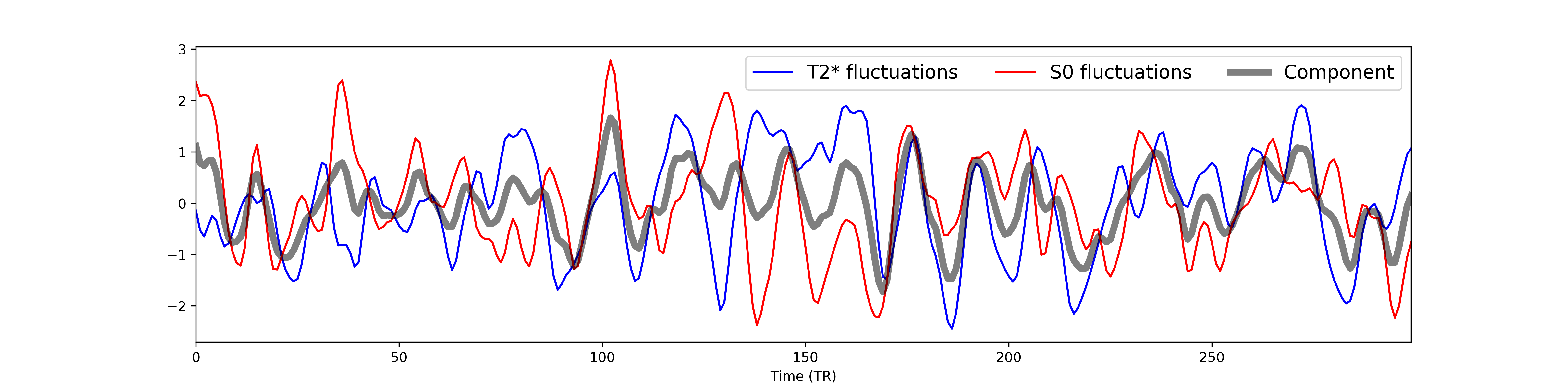
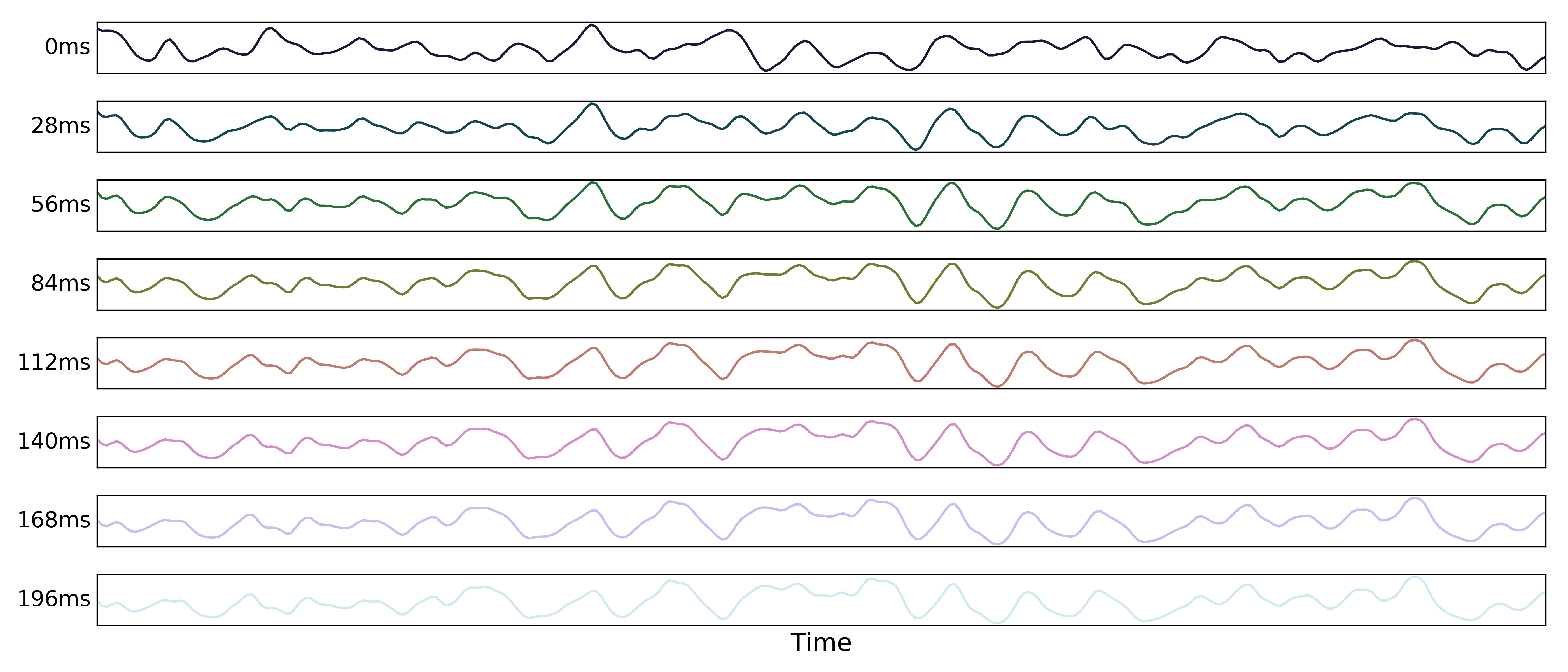
We also simulate multi-echo data for a single voxel with both the T2* and S0 fluctuations. Here we show time series for a subset of echo times.
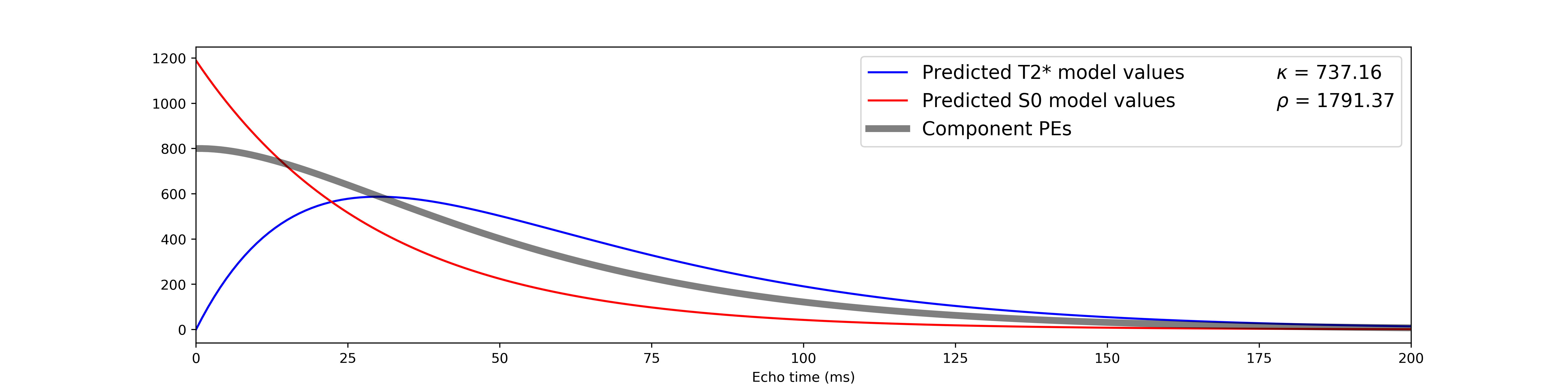
We then fit parameter estimates for echo data against the component time
series.
We can compare predicted T2* and S0 model values against the parameter estimates
in order to calculate single-voxel  and
and  values.
Note that the metric values are extremely high, due to the inflated
degrees of freedom resulting from using so many echoes in the simulations.
You may also notice that, despite the fact that T2* and S0 fluctuate the same
amount and that both contributed equally to the component, is
much higher than .
values.
Note that the metric values are extremely high, due to the inflated
degrees of freedom resulting from using so many echoes in the simulations.
You may also notice that, despite the fact that T2* and S0 fluctuate the same
amount and that both contributed equally to the component, is
much higher than .