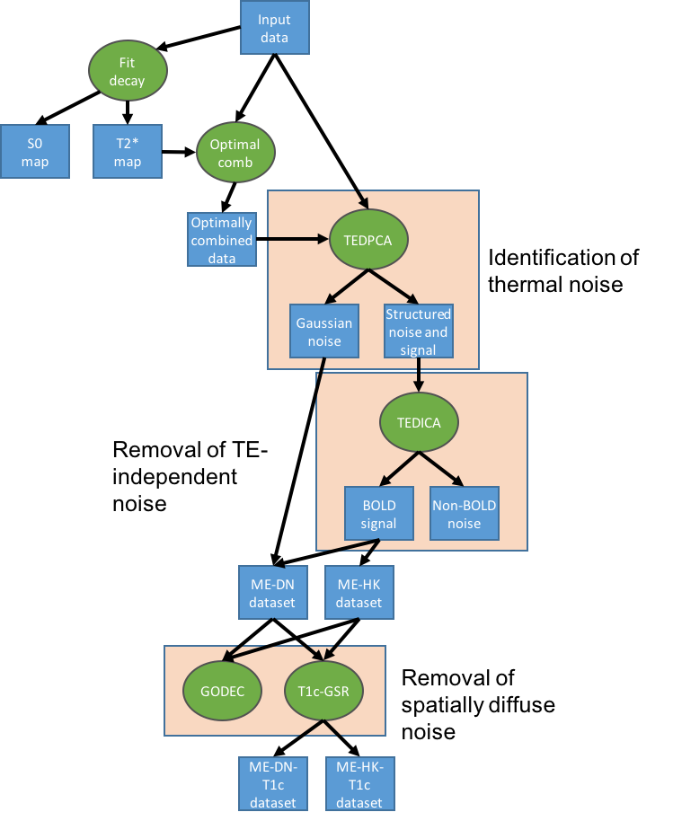
Processing pipeline details
tedana works by decomposing multi-echo BOLD data via PCA and ICA.
The resulting components are then analyzed to determine whether they are
TE-dependent or -independent.
TE-dependent components are classified as BOLD, while TE-independent components
are classified as non-BOLD, and are discarded as part of data cleaning.
In tedana, we take the time series from all the collected TEs, combine them,
and decompose the resulting data into components that can be classified as BOLD
or non-BOLD.
This is performed in a series of steps, including:
- Principal components analysis
- Independent components analysis
- Component classification
Multi-echo data
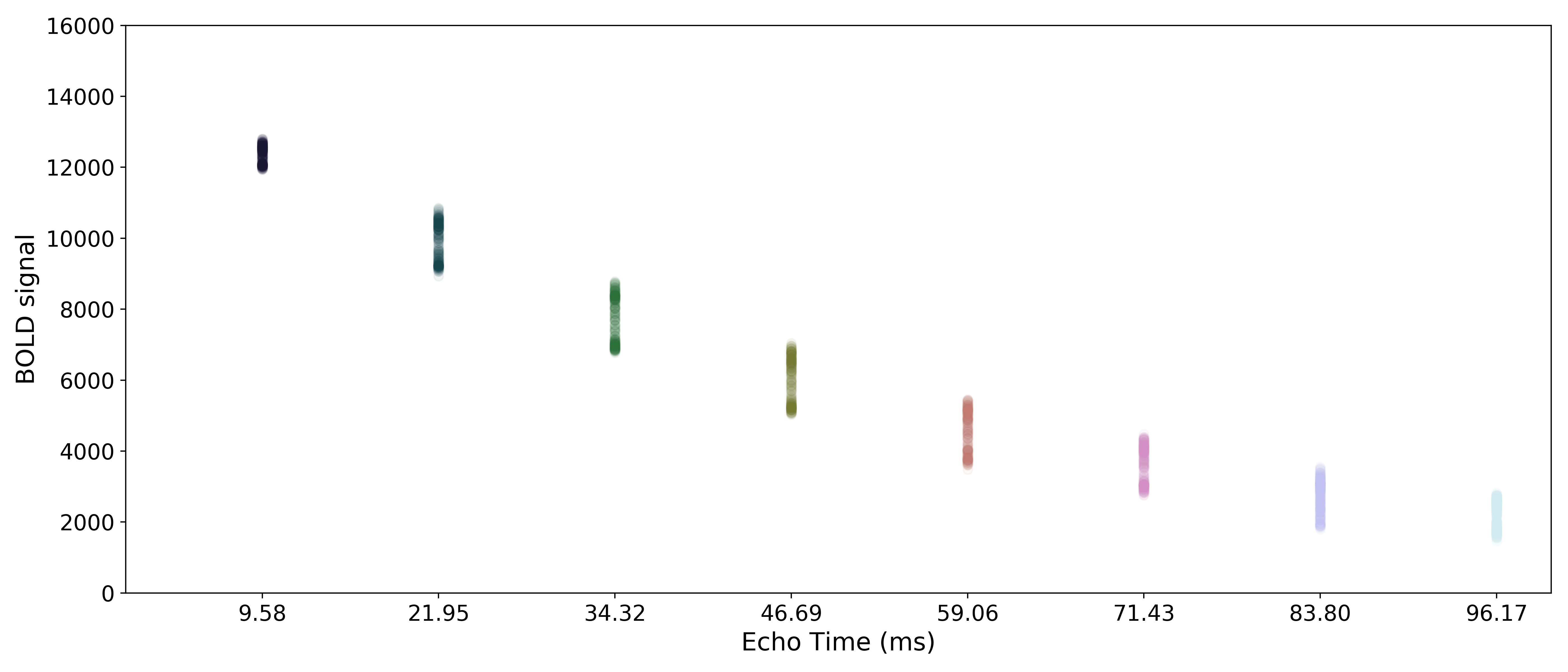
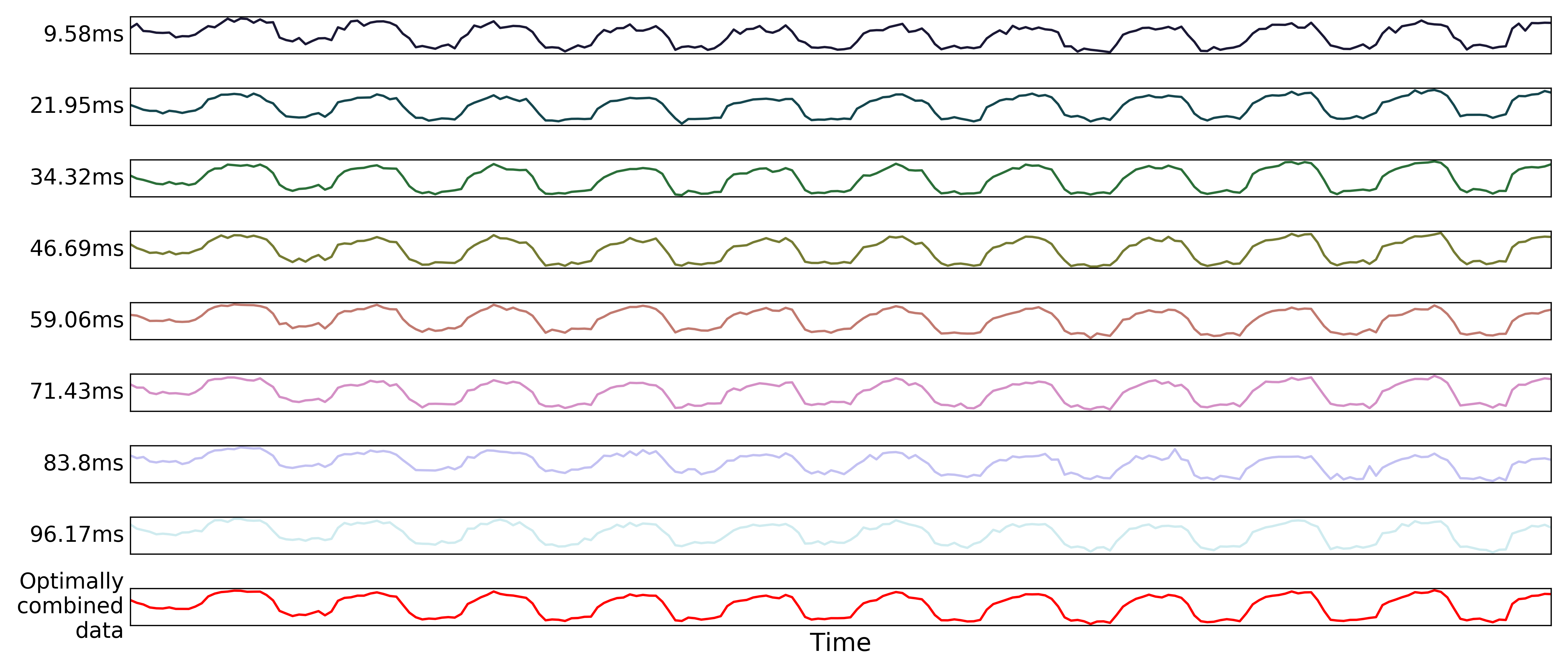
Here are the echo-specific time series for a single voxel in an example resting-state scan with 5 echoes.
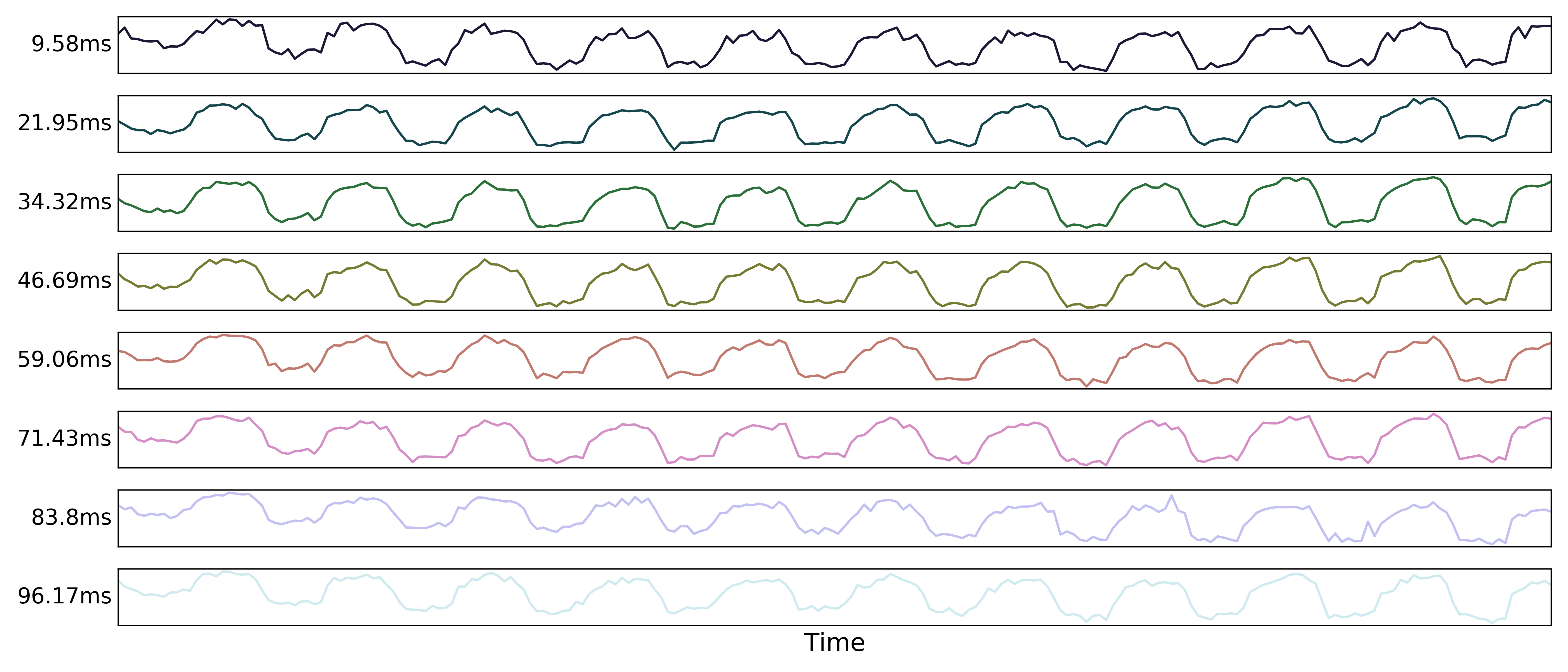
The values across volumes for this voxel scale with echo time in a predictable manner.
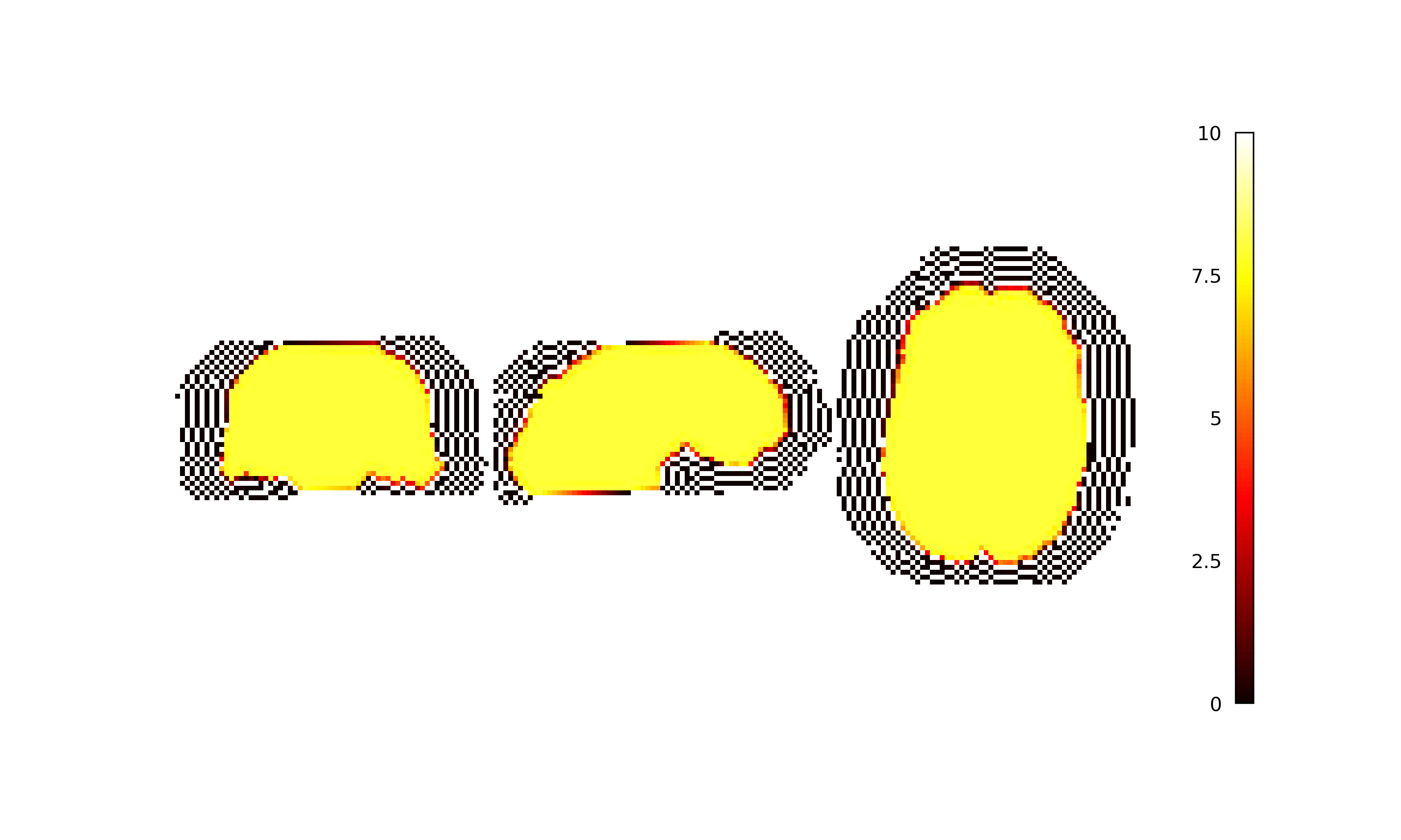
Adaptive mask generation
Longer echo times are more susceptible to signal dropout, which means that
certain brain regions (e.g., orbitofrontal cortex, temporal poles) will only
have good signal for some echoes.
In order to avoid using bad signal from affected echoes in calculating
 and
and  for a given voxel,
 tedana generates an
adaptive mask, where the value for each voxel is the number of echoes with
“good” signal.
When and are calculated below, each voxel’s values
are only calculated from the first  echoes, where is the
value for that voxel in the adaptive mask.
echoes, where is the
value for that voxel in the adaptive mask.
Note
tedana allows users to provide their own mask.
The adaptive mask will be computed on this explicit mask, and may reduce
it further based on the data.
If a mask is not provided, tedana runs nilearn.masking.compute_epi_mask
on the first echo’s data to derive a mask prior to adaptive masking.
The workflow does this because the adaptive mask generation function
sometimes identifies almost the entire bounding box as “brain”, and
compute_epi_mask restricts analysis to a more reasonable area.
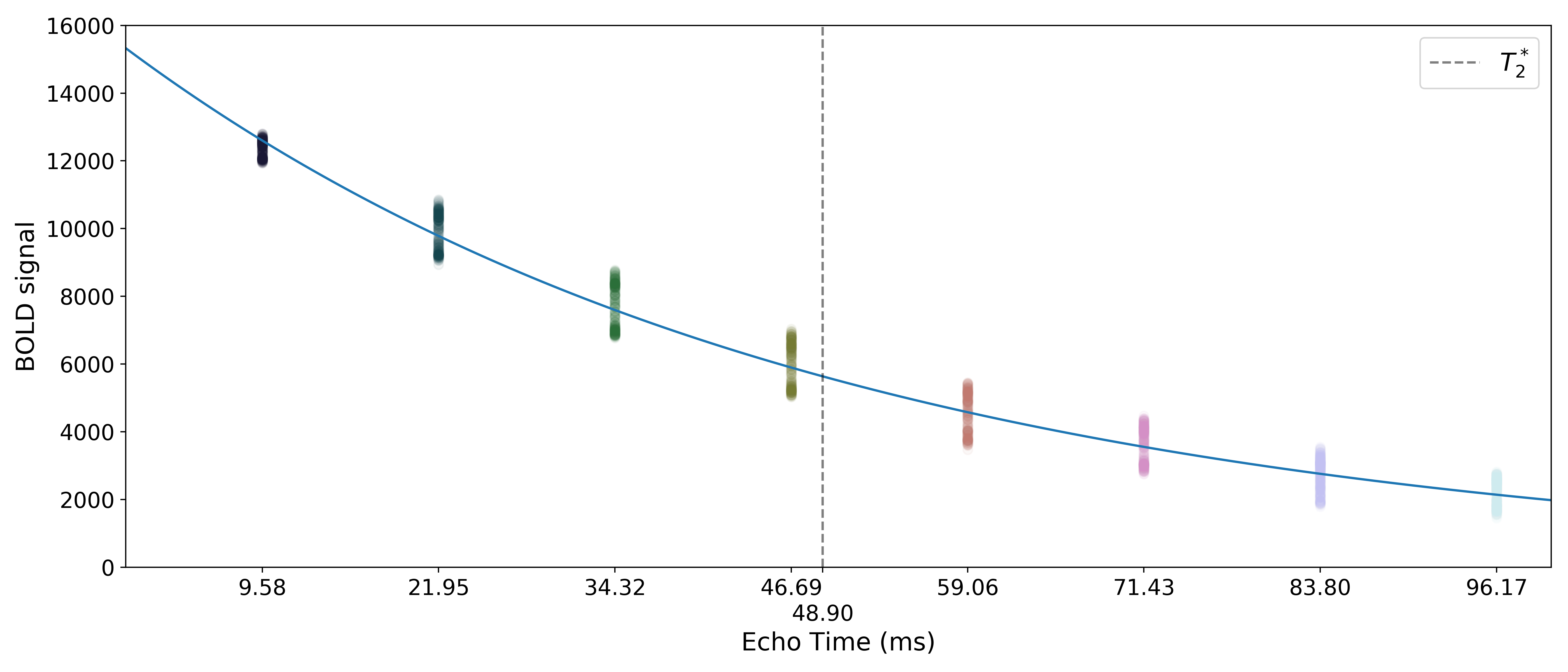
Monoexponential decay model fit
The next step is to fit a monoexponential decay model to the data in order to
estimate voxel-wise and  .
While and in fact fluctuate over time, estimating
them on a volume-by-volume basis with only a small number of echoes is not
feasible (i.e., the estimates would be extremely noisy).
As such, we estimate average and maps and use those
throughout the workflow.
.
While and in fact fluctuate over time, estimating
them on a volume-by-volume basis with only a small number of echoes is not
feasible (i.e., the estimates would be extremely noisy).
As such, we estimate average and maps and use those
throughout the workflow.
In order to make it easier to fit the decay model to the data, tedana
transforms the data.
The BOLD data are transformed as  , where
  is the BOLD signal.
The echo times are also multiplied by -1.
is the BOLD signal.
The echo times are also multiplied by -1.
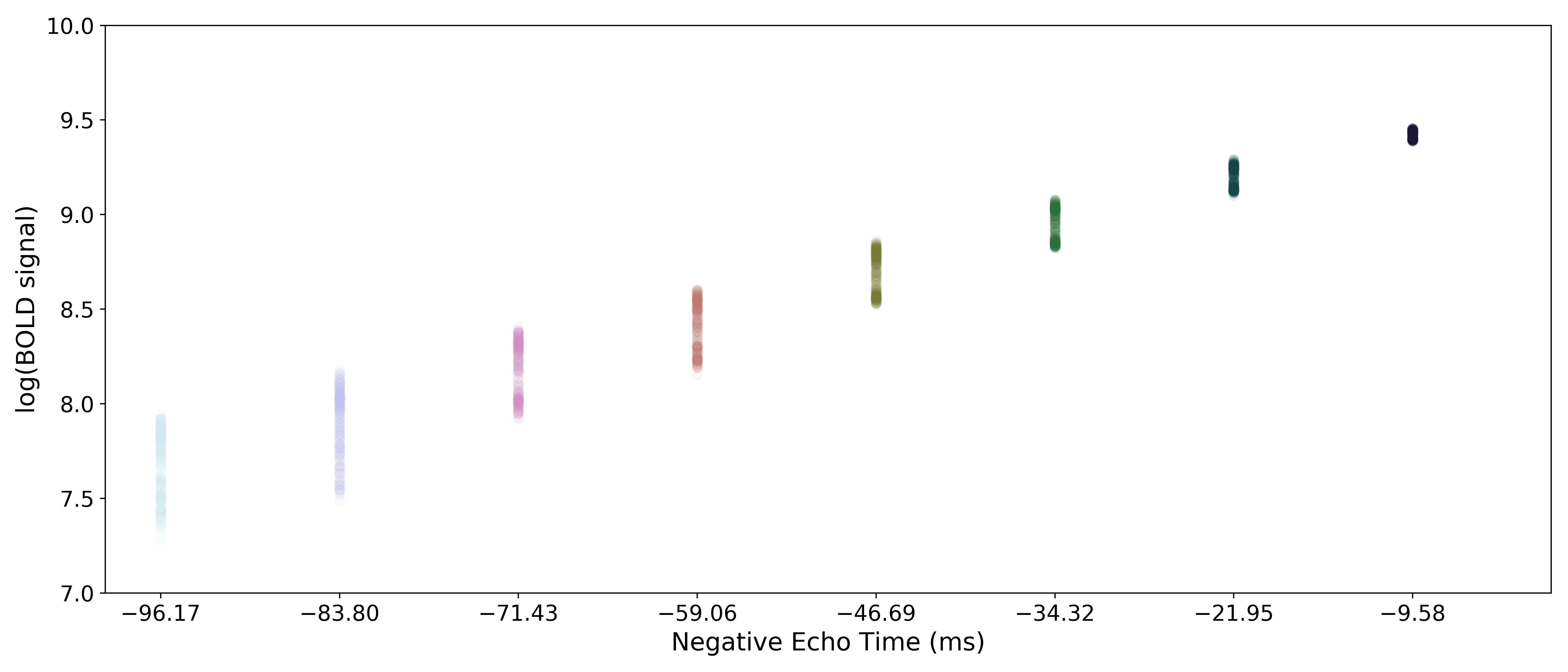
A simple line can then be fit to the transformed data with linear regression. For the sake of this introduction, we can assume that the example voxel has good signal in all five echoes (i.e., the adaptive mask has a value of 5 at this voxel), so the line is fit to all available data.
Note
tedana actually performs and uses two sets of / model fits.
In one case, tedana estimates and for voxels with good signal in at
least two echoes.
The resulting “limited” and maps are used throughout
most of the pipeline.
In the other case, tedana estimates and for voxels
with good data in only one echo as well, but uses the first two echoes for those voxels.
The resulting “full” and maps are used to generate the
optimally combined data.
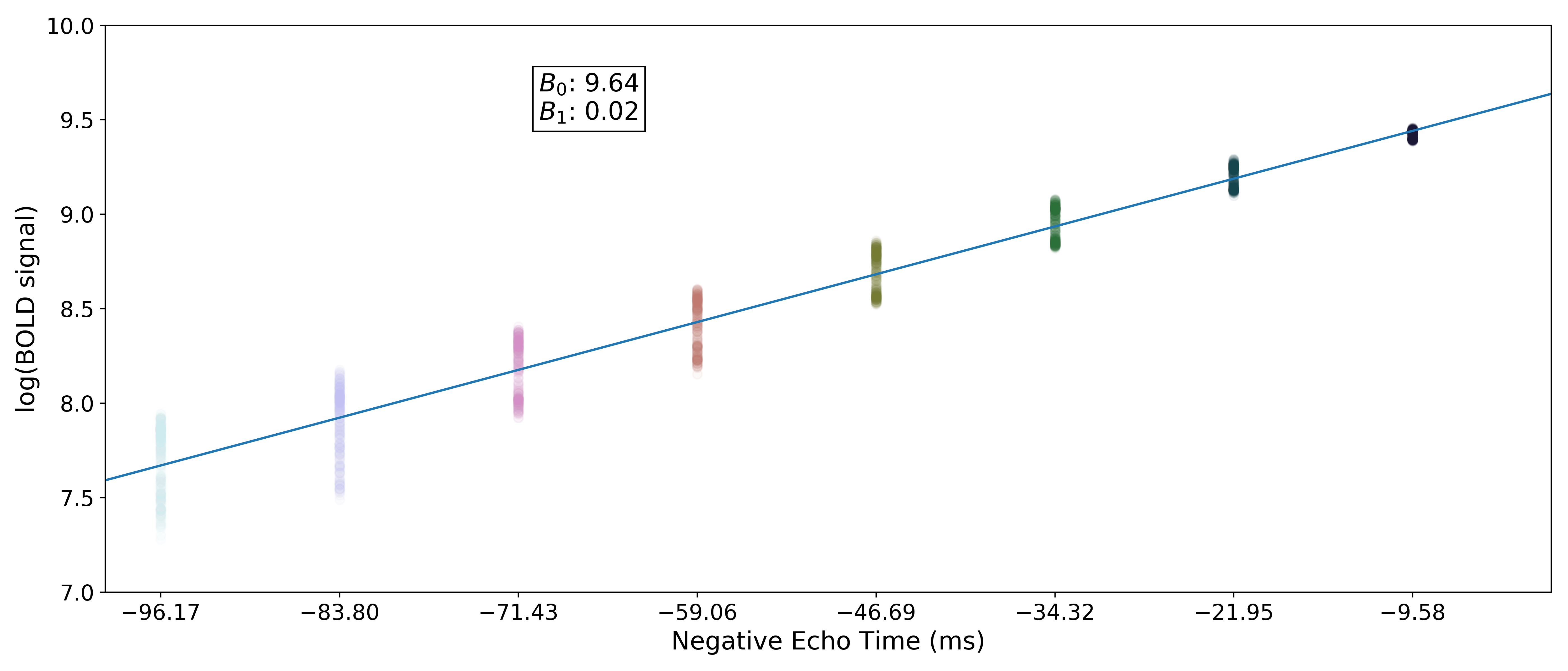
The values of interest for the decay model, and ,
are then simple transformations of the line’s intercept ( ) and
slope (
) and
slope ( ), respectively:


The resulting values can be used to show the fitted monoexponential decay model on the original data.
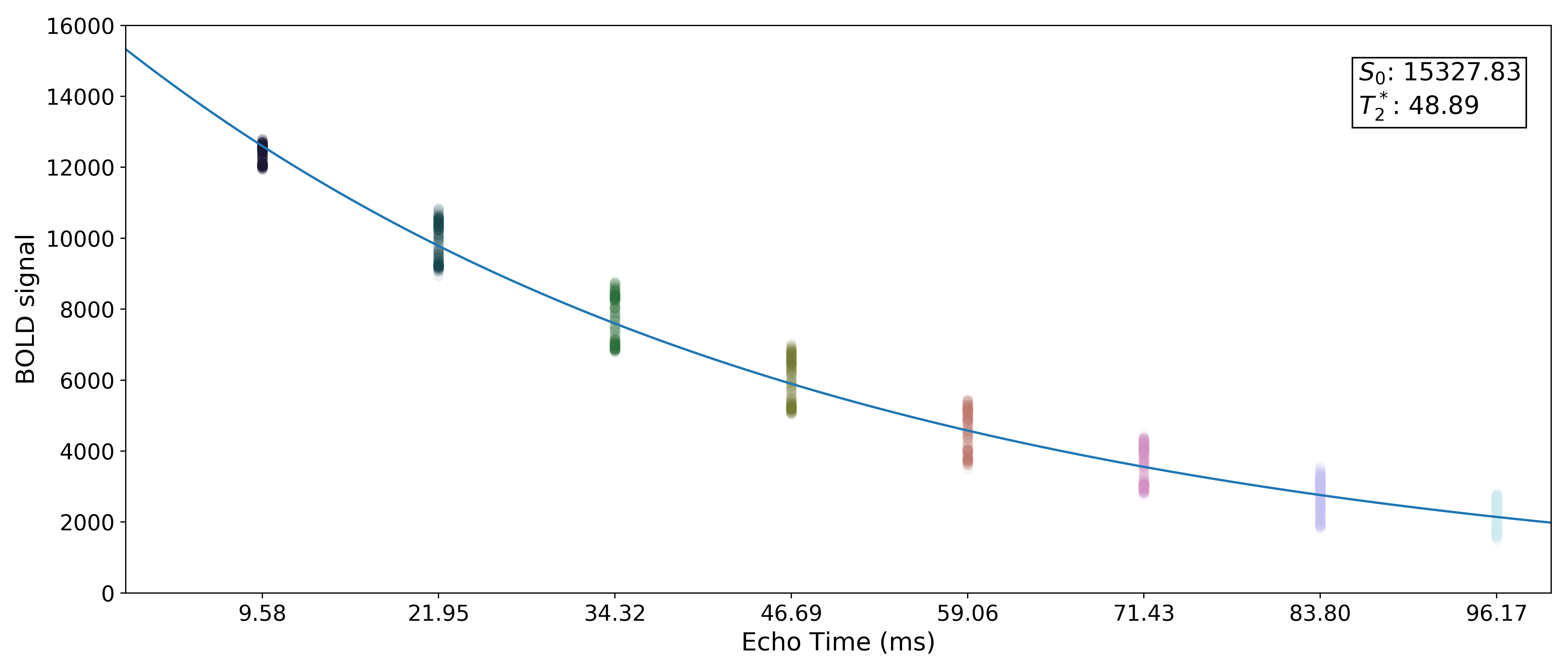
We can also see where lands on this curve.
Optimal combination
Using the estimates, tedana combines signal across echoes using a
weighted average.
The echoes are weighted according to the formula
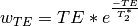
The weights are then normalized across echoes. For the example voxel, the resulting weights are:
The distribution of values for the optimally combined data lands somewhere between the distributions for other echoes.
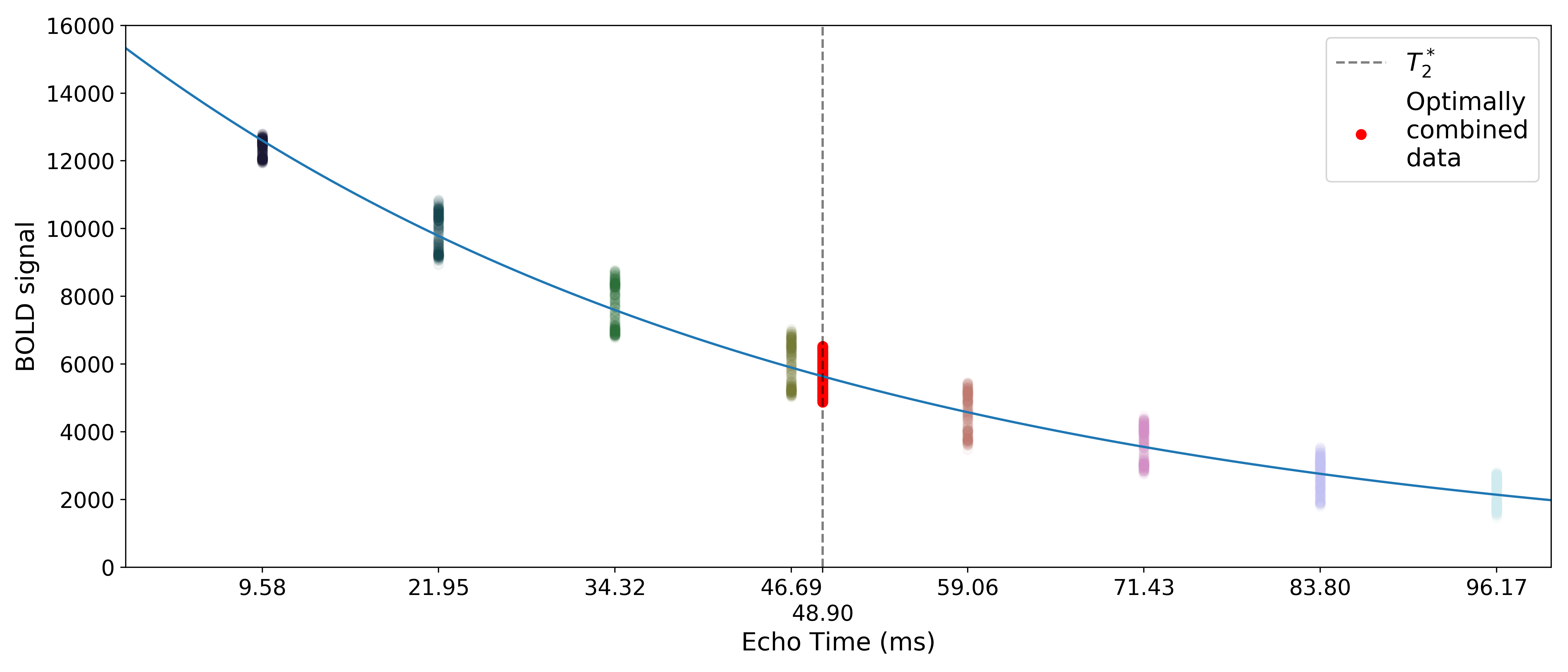
The time series for the optimally combined data also looks like a combination of the other echoes (which it is).
Note
An alternative method for optimal combination that
does not use , is the parallel-acquired inhomogeneity
desensitized (PAID) ME-fMRI combination method (Poser et al., 2006).
This method specifically assumes that noise in the acquired echoes is “isotopic and
homogeneous throughout the image,” meaning it should be used on smoothed data.
As we do not recommend performing tedana denoising on smoothed data,
we discourage using PAID within the tedana workflow.
We do, however, make it accessible as an alternative combination method
in the t2smap workflow.
TEDPCA
The next step is to dimensionally reduce the data with TE-dependent principal components analysis (PCA). The goal of this step is to make it easier for the later ICA decomposition to converge. Dimensionality reduction is a common step prior to ICA. TEDPCA applies PCA to the optimally combined data in order to decompose it into component maps and time series. Here we can see time series for some example components (we don’t really care about the maps):
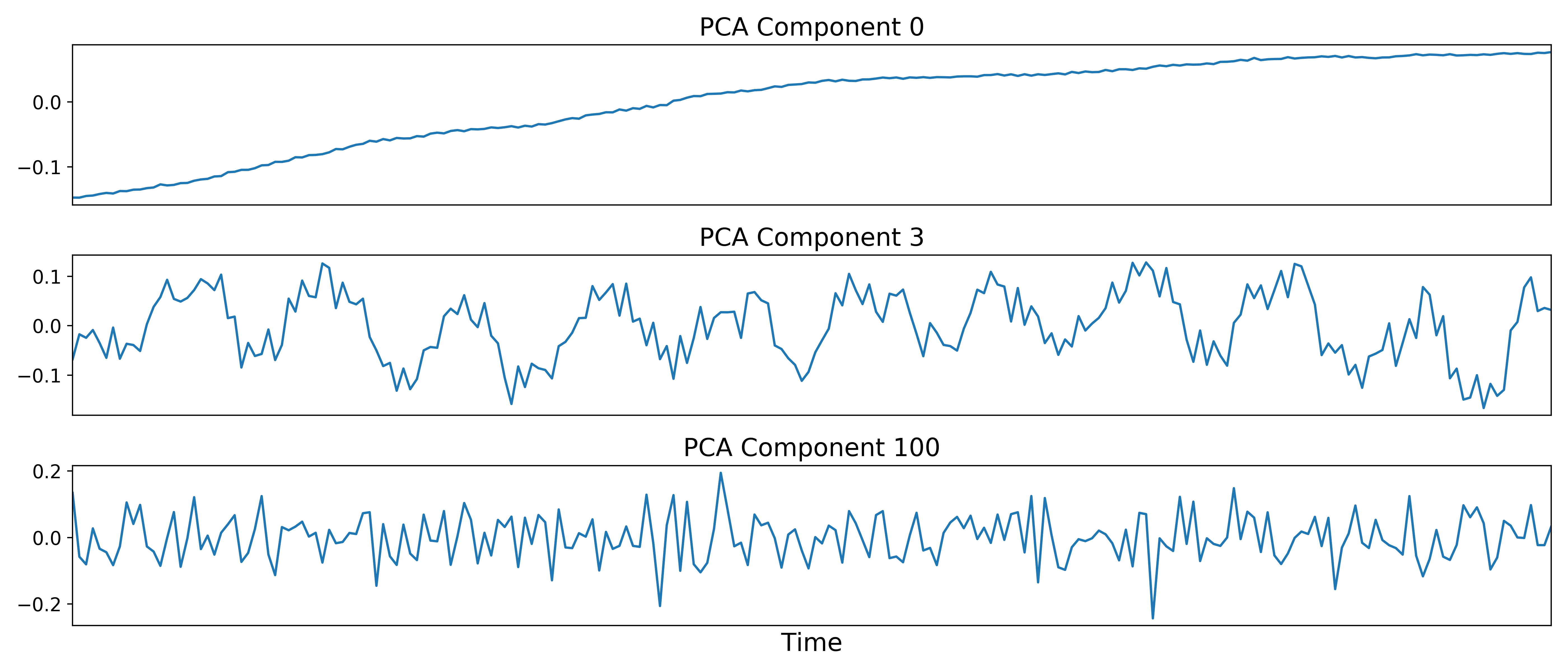
These components are subjected to component selection, the specifics of which vary according to algorithm.
In the simplest approach, tedana uses Minka’s MLE to estimate the
dimensionality of the data, which disregards low-variance components.
A more complicated approach involves applying a decision tree to identify and discard PCA components which, in addition to not explaining much variance, are also not significantly TE-dependent (i.e., have low Kappa) or TE-independent (i.e., have low Rho).
Note
This process (also performed in TEDICA) can be broadly separated into three steps: decomposition, metric calculation, and component selection. Decomposition identifies components in the data. Metric calculation derives relevant summary statistics for each component. Component selection uses the summary statistics to identify components that should be kept or discarded.
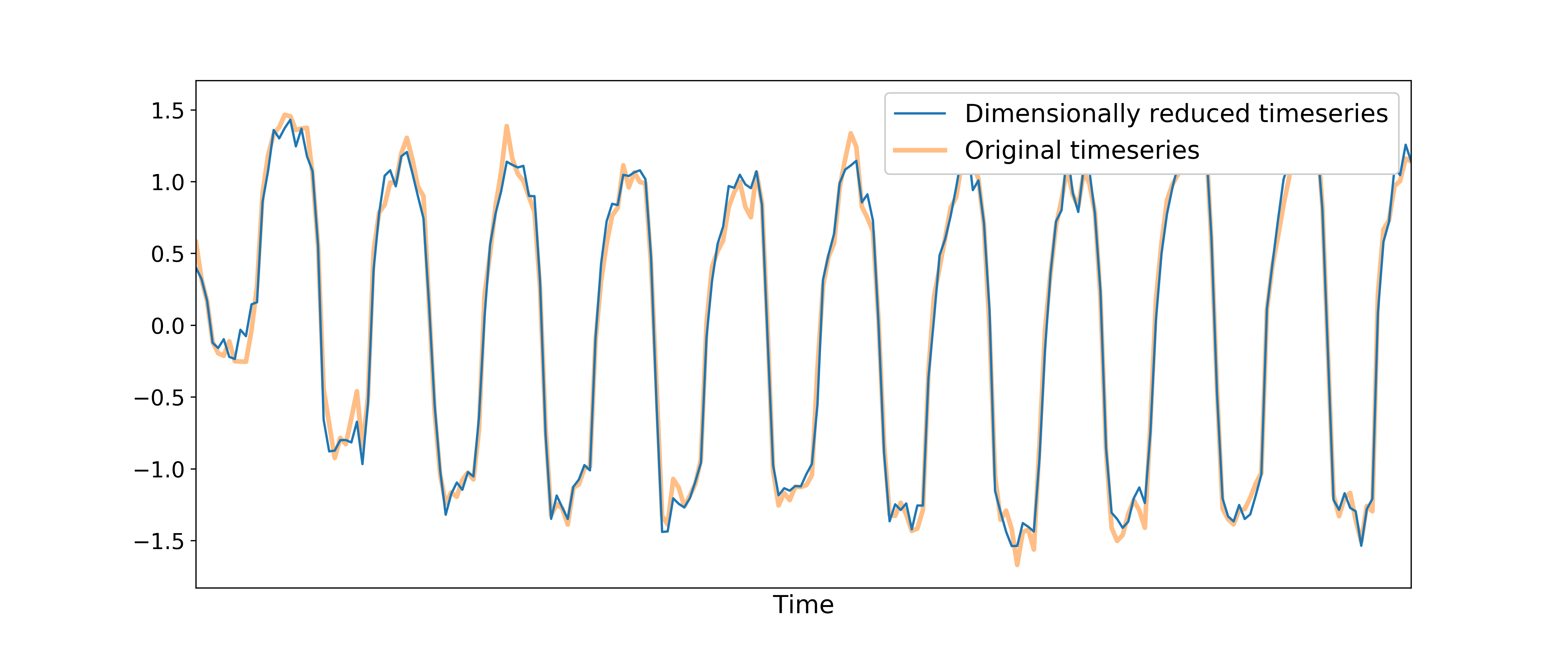
After component selection is performed, the retained components and their associated betas are used to reconstruct the optimally combined data, resulting in a dimensionally reduced version of the dataset.
TEDICA
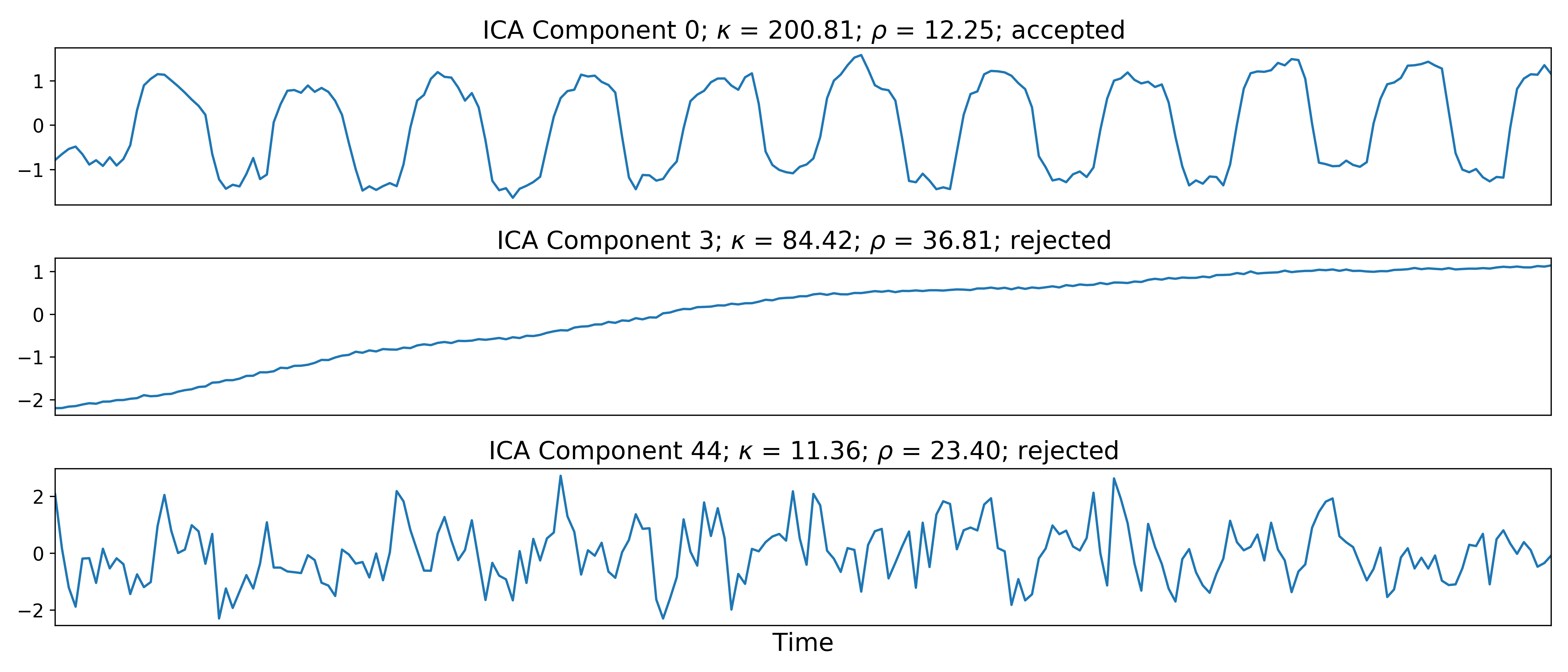
Next, tedana applies TE-dependent independent components analysis (ICA) in
order to identify and remove TE-independent (i.e., non-BOLD noise) components.
The dimensionally reduced optimally combined data are first subjected to ICA in
order to fit a mixing matrix to the whitened data.
Linear regression is used to fit the component time series to each voxel in each echo from the original, echo-specific data. This way, low-variance information (originally discarded by TEDPCA) is retained in the data, but is ignored by the TEDICA process. This results in echo- and voxel-specific betas for each of the components.
TE-dependence ( ) and TE-independence () models can then
be fit to these betas.
For more information on how these models are estimated, see TE (In)Dependence Models.
These models allow calculation of F-statistics for the and
models (referred to as
) and TE-independence () models can then
be fit to these betas.
For more information on how these models are estimated, see TE (In)Dependence Models.
These models allow calculation of F-statistics for the and
models (referred to as  and
and  , respectively).
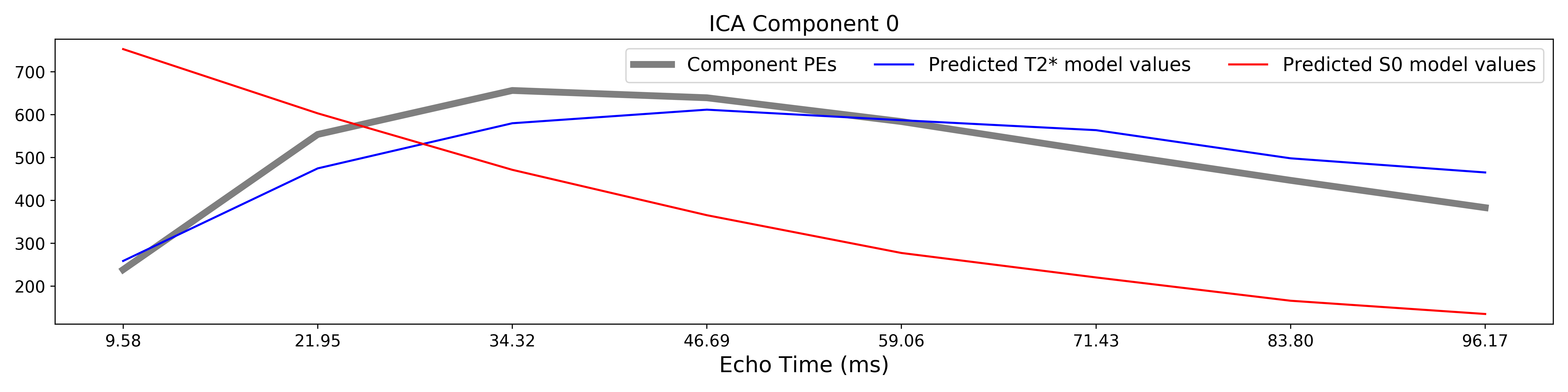
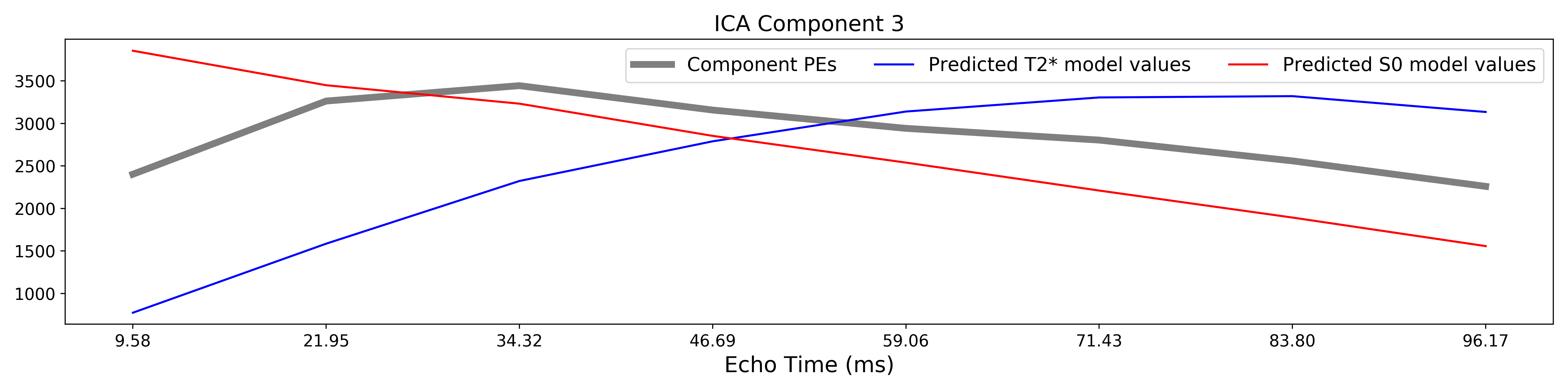
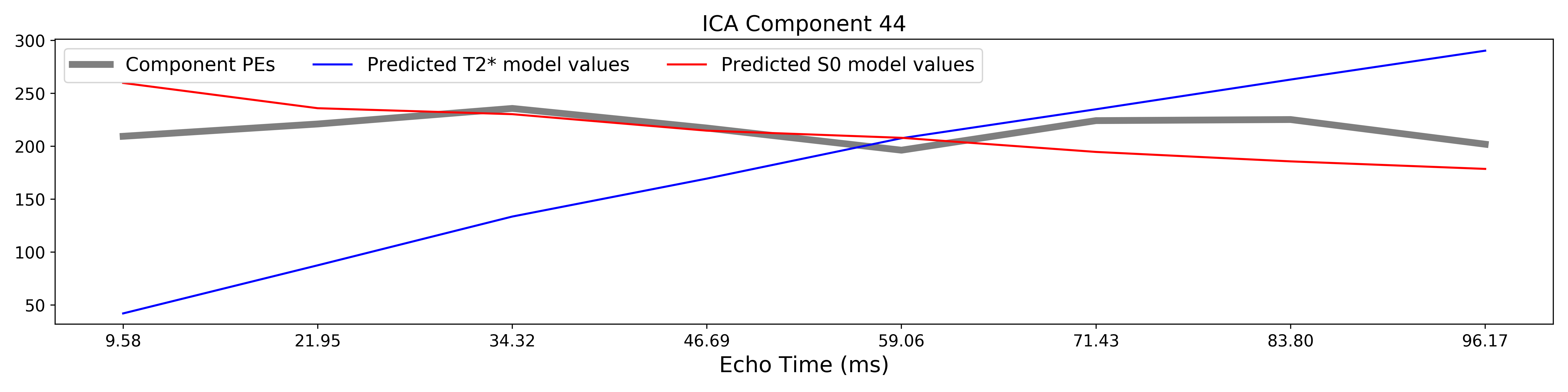
A decision tree is applied to , , and other metrics in order to
classify ICA components as TE-dependent (BOLD signal), TE-independent
(non-BOLD noise), or neither (to be ignored).
The actual decision tree is dependent on the component selection algorithm employed.
tedana includes two options: kundu_v2_5 (which uses hardcoded thresholds
applied to each of the metrics) and kundu_v3_2 (which trains a classifier to
select components).
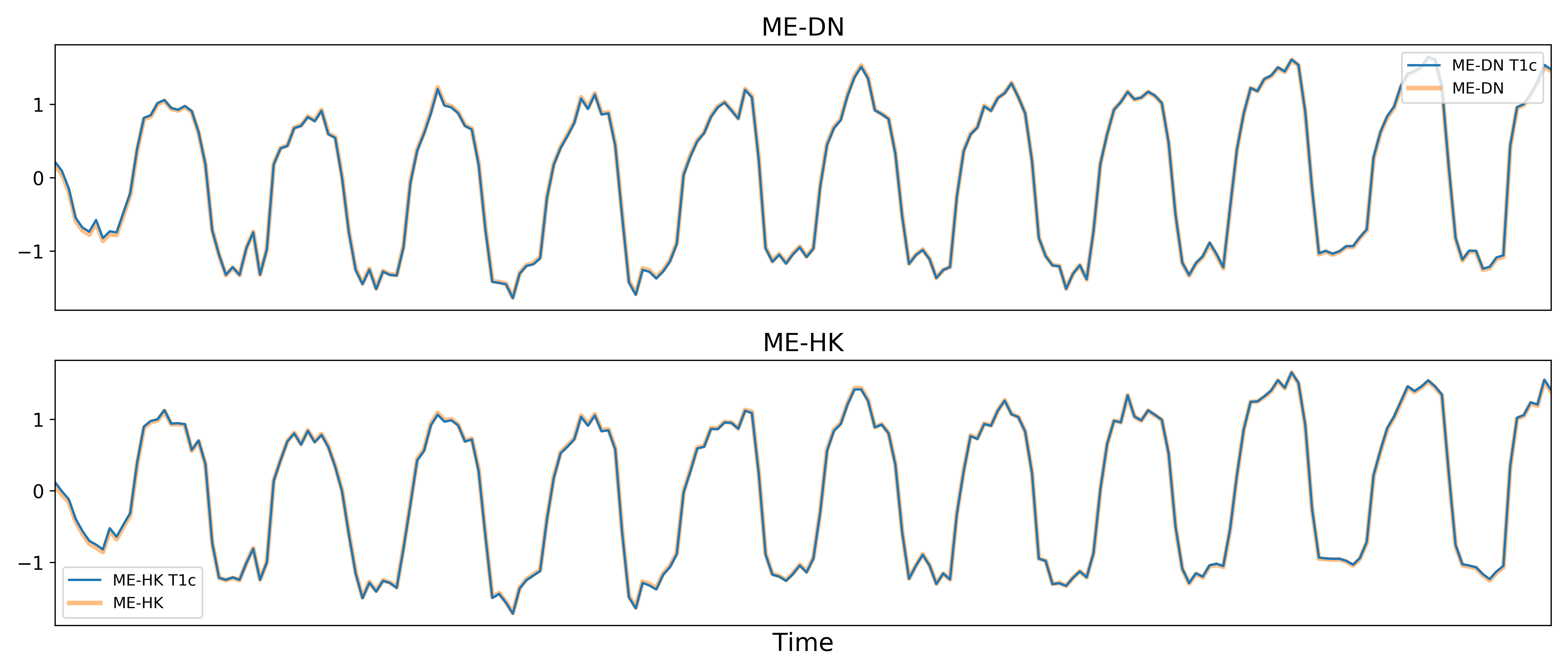
Removal of spatially diffuse noise (optional)
Due to the constraints of ICA, TEDICA is able to identify and remove spatially
localized noise components, but it cannot identify components that are spread
out throughout the whole brain. See Power et al. (2018) for more information
about this issue.
One of several post-processing strategies may be applied to the ME-DN or ME-HK
datasets in order to remove spatially diffuse (ostensibly respiration-related)
noise.
Methods which have been employed in the past include global signal
regression (GSR), T1c-GSR, anatomical CompCor, Go Decomposition (GODEC), and
robust PCA.
Currently, tedana implements GSR and T1c-GSR.