Outputs of tedana
tedana derivatives
| Filename | Content |
|---|---|
| t2sv.nii | Limited estimated T2* 3D map. The difference between the limited and full maps is that, for voxels affected by dropout where only one echo contains good data, the full map uses the single echo’s value while the limited map has a NaN. |
| s0v.nii | Limited S0 3D map. The difference between the limited and full maps is that, for voxels affected by dropout where only one echo contains good data, the full map uses the single echo’s value while the limited map has a NaN. |
| ts_OC.nii | Optimally combined time series. |
| dn_ts_OC.nii | Denoised optimally combined time series. Recommended dataset for analysis. |
| lowk_ts_OC.nii | Combined time series from rejected components. |
| midk_ts_OC.nii | Combined time series from “mid-k” rejected components. |
| hik_ts_OC.nii | High-kappa time series. This dataset does not include thermal noise or low variance components. Not the recommended dataset for analysis. |
| comp_table_pca.txt | TEDPCA component table. A tab-delimited file with summary metrics and inclusion/exclusion information for each component from the PCA decomposition. |
| mepca_mix.1D | Mixing matrix (component time series) from PCA decomposition. |
| meica_mix.1D | Mixing matrix (component time series) from ICA decomposition. The only differences between this mixing matrix and the one above are that components may be sorted differently and signs of time series may be flipped. |
| betas_OC.nii | Full ICA coefficient feature set. |
| betas_hik_OC.nii | High-kappa ICA coefficient feature set |
| feats_OC2.nii | Z-normalized spatial component maps |
| comp_table_ica.txt | TEDICA component table. A tab-delimited file with summary metrics and inclusion/exclusion information for each component from the ICA decomposition. |
| report.txt | A summary report for the workflow with relevant citations. |
If verbose is set to True:
| Filename | Content |
|---|---|
| t2ss.nii | Voxel-wise T2* estimates using ascending numbers of echoes, starting with 2. |
| s0vs.nii | Voxel-wise S0 estimates using ascending numbers of echoes, starting with 2. |
| t2svG.nii | Full T2* map/time series. The difference between the limited and full maps is that, for voxels affected by dropout where only one echo contains good data, the full map uses the single echo’s value while the limited map has a NaN. Only used for optimal combination. |
| s0vG.nii | Full S0 map/time series. Only used for optimal combination. |
| hik_ts_e[echo].nii | High-Kappa time series for echo number echo |
| midk_ts_e[echo].nii | Mid-Kappa time series for echo number echo |
| lowk_ts_e[echo].nii | Low-Kappa time series for echo number echo |
| dn_ts_e[echo].nii | Denoised time series for echo number echo |
If gscontrol includes ‘gsr’:
| Filename | Content |
|---|---|
| T1gs.nii | Spatial global signal |
| glsig.1D | Time series of global signal from optimally combined data. |
| tsoc_orig.nii | Optimally combined time series with global signal retained. |
| tsoc_nogs.nii | Optimally combined time series with global signal removed. |
If gscontrol includes ‘t1c’:
| Filename | Content |
|---|---|
| sphis_hik.nii | T1-like effect |
| hik_ts_OC_T1c.nii | T1 corrected high-kappa time series by regression |
| dn_ts_OC_T1c.nii | T1 corrected denoised time series |
| betas_hik_OC_T1c.nii | T1-GS corrected high-kappa components |
| meica_mix_T1c.1D | T1-GS corrected mixing matrix |
Component tables
TEDPCA and TEDICA use tab-delimited tables to track relevant metrics, component classifications, and rationales behind classifications. TEDPCA rationale codes start with a “P”, while TEDICA codes start with an “I”.
| Classification | Description |
|---|---|
| accepted | BOLD-like components retained in denoised and high-Kappa data |
| rejected | Non-BOLD components removed from denoised and high-Kappa data |
| ignored | Low-variance components ignored in denoised, but not high-Kappa, data |
TEDPCA codes
| Code | Classification | Description |
|---|---|---|
| P001 | rejected | Low Rho, Kappa, and variance explained |
| P002 | rejected | Low variance explained |
| P003 | rejected | Kappa equals fmax |
| P004 | rejected | Rho equals fmax |
| P005 | rejected | Cumulative variance explained above 95% (only in stabilized PCA decision tree) |
| P006 | rejected | Kappa below fmin (only in stabilized PCA decision tree) |
| P007 | rejected | Rho below fmin (only in stabilized PCA decision tree) |
TEDICA codes
| Code | Classification | Description |
|---|---|---|
| I001 | rejected|accepted | Manual classification |
| I002 | rejected | Rho greater than Kappa |
| I003 | rejected | More significant voxels in S0 model than R2 model |
| I004 | rejected | S0 Dice is higher than R2 Dice and high variance explained |
| I005 | rejected | Noise F-value is higher than signal F-value and high variance explained |
| I006 | ignored | No good components found |
| I007 | rejected | Mid-Kappa component |
| I008 | ignored | Low variance explained |
| I009 | rejected | Mid-Kappa artifact type A |
| I010 | rejected | Mid-Kappa artifact type B |
| I011 | ignored | ign_add0 |
| I012 | ignored | ign_add1 |
Citable workflow summaries
tedana generates a report for the workflow, customized based on the parameters used and including relevant citations.
The report is saved in a plain-text file, report.txt, in the output directory.
An example report
TE-dependence analysis was performed on input data. An initial mask was generated from the first echo using nilearn’s compute_epi_mask function. An adaptive mask was then generated, in which each voxel’s value reflects the number of echoes with ‘good’ data. A monoexponential model was fit to the data at each voxel using log-linear regression in order to estimate T2* and S0 maps. For each voxel, the value from the adaptive mask was used to determine which echoes would be used to estimate T2* and S0. Multi-echo data were then optimally combined using the ‘t2s’ (Posse et al., 1999) combination method. Global signal regression was applied to the multi-echo and optimally combined datasets. Principal component analysis followed by the Kundu component selection decision tree (Kundu et al., 2013) was applied to the optimally combined data for dimensionality reduction. Independent component analysis was then used to decompose the dimensionally reduced dataset. A series of TE-dependence metrics were calculated for each ICA component, including Kappa, Rho, and variance explained. Next, component selection was performed to identify BOLD (TE-dependent), non-BOLD (TE-independent), and uncertain (low-variance) components using the Kundu decision tree (v2.5; Kundu et al., 2013). T1c global signal regression was then applied to the data in order to remove spatially diffuse noise.
This workflow used numpy (Van Der Walt, Colbert, & Varoquaux, 2011), scipy (Jones et al., 2001), pandas (McKinney, 2010), scikit-learn (Pedregosa et al., 2011), nilearn, and nibabel (Brett et al., 2019).
This workflow also used the Dice similarity index (Dice, 1945; Sørensen, 1948).
References
Brett, M., Markiewicz, C. J., Hanke, M., Côté, M.-A., Cipollini, B., McCarthy, P., … freec84. (2019, May 28). nipy/nibabel. Zenodo. http://doi.org/10.5281/zenodo.3233118
Dice, L. R. (1945). Measures of the amount of ecologic association between species. Ecology, 26(3), 297-302.
Jones E, Oliphant E, Peterson P, et al. SciPy: Open Source Scientific Tools for Python, 2001-, http://www.scipy.org/
Kundu, P., Brenowitz, N. D., Voon, V., Worbe, Y., Vértes, P. E., Inati, S. J., … & Bullmore, E. T. (2013). Integrated strategy for improving functional connectivity mapping using multiecho fMRI. Proceedings of the National Academy of Sciences, 110(40), 16187-16192.
McKinney, W. (2010, June). Data structures for statistical computing in python. In Proceedings of the 9th Python in Science Conference (Vol. 445, pp. 51-56).
Pedregosa, F., Varoquaux, G., Gramfort, A., Michel, V., Thirion, B., Grisel, O., … & Vanderplas, J. (2011). Scikit-learn: Machine learning in Python. Journal of machine learning research, 12(Oct), 2825-2830.
Posse, S., Wiese, S., Gembris, D., Mathiak, K., Kessler, C., Grosse‐Ruyken, M. L., … & Kiselev, V. G. (1999). Enhancement of BOLD‐contrast sensitivity by single‐shot multi‐echo functional MR imaging. Magnetic Resonance in Medicine: An Official Journal of the International Society for Magnetic Resonance in Medicine, 42(1), 87-97.
Sørensen, T. J. (1948). A method of establishing groups of equal amplitude in plant sociology based on similarity of species content and its application to analyses of the vegetation on Danish commons. I kommission hos E. Munksgaard.
Van Der Walt, S., Colbert, S. C., & Varoquaux, G. (2011). The NumPy array: a structure for efficient numerical computation. Computing in Science & Engineering, 13(2), 22.
Visual reports
Static visual reports can be generated by using the --png flag when calling
tedana from the command line.
Images are created and placed within the output directory, in a folder labeled
figures.
These reports consist of three main types of images.
Component Images
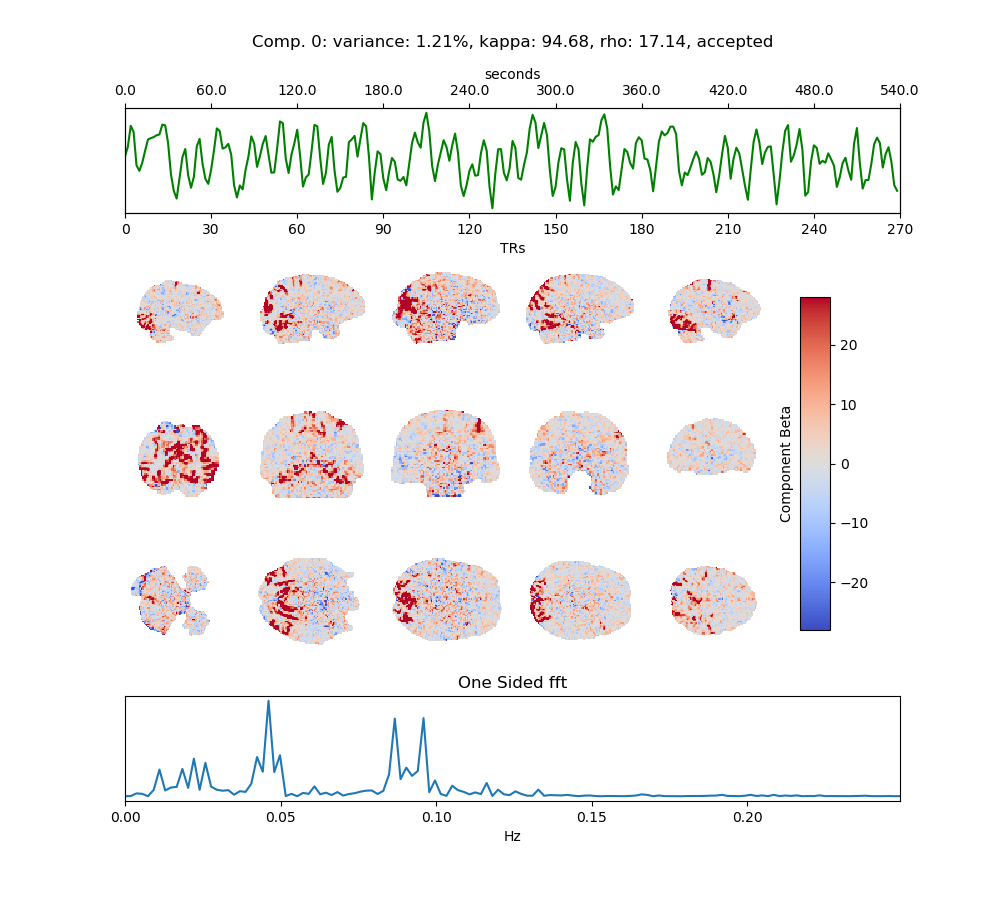
For each component identified by tedana, a single image will be created. Above is an example of an accepted component. These are designed for an up-close inspection of both the spatial and temporal aspects of the component, as well as ancillary information.
The title of the plot provides information about variance, kappa and rho values as well as the reasons for rejection, if any (see above for codes).
Below this is the component timeseries, color coded on the basis of its classification. Green for accepted, Red for rejected, Black for ignored or unclassified.
Slices are then selected from sagittal, axial and coronal planes, to highlight the component pattern. By default these images used the red-blue colormap and are scaled to 10% of the max beta value.
Note
You can select your own colormap to use by specifying its name when calling
tedana with --png-cmap.
For example, to use the bone colormap, you would add --png-cmap bone.
Finally, the bottom of the image shows the Fast Fourier Transform of the component timeseries.
Tip: Look for your fundamental task frequencies here!
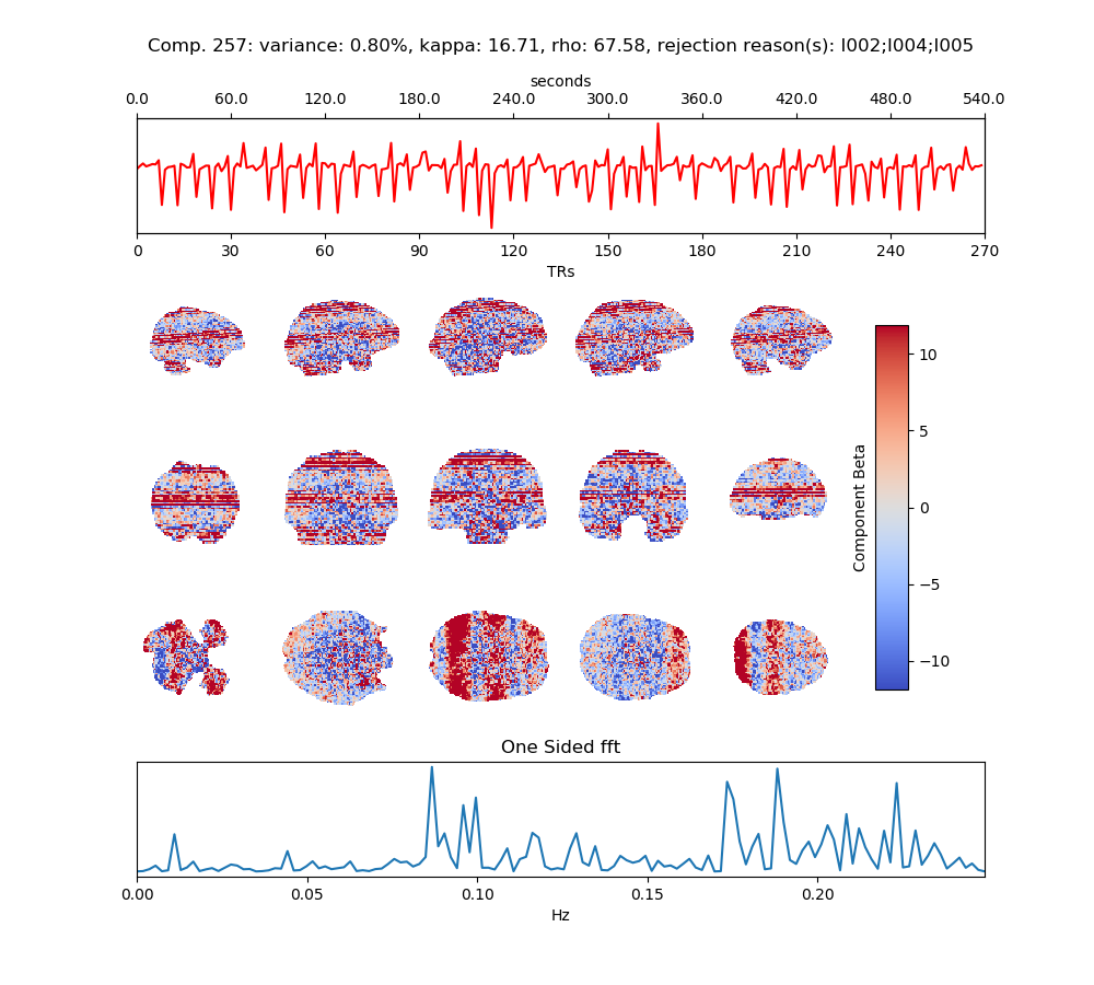
Above, you can review a component that was rejected. In this case, the subject moved each time the task was performed - which affected single slices of the fMRI volume. This scan used multiband imaging (collecting multiple slices at once), so the motion artifact occurs in more than once slice.
Kappa vs Rho Scatter Plot
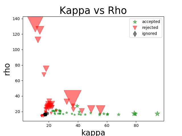
This diagnostic plot shows the relationship between kappa and rho values for each component.
This can be useful for getting a big picture view of your data or for comparing denoising performance with various fMRI sequences.
Double Pie Chart
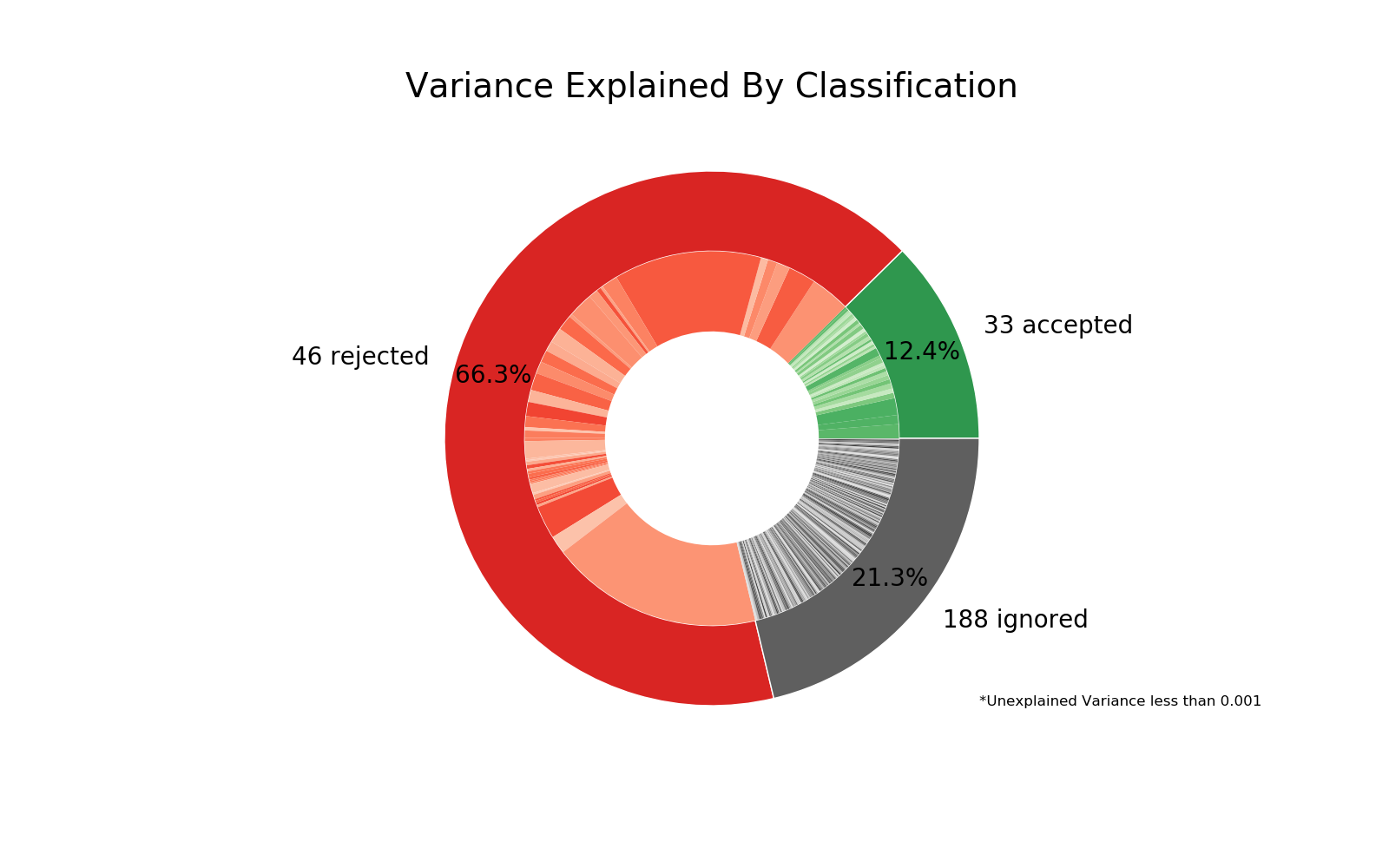
This diagnostic plot shows the relative variance explained by each classification type in the outer ring, with individual components on the inner ring. If a low amount of variance is explained, this will be shown as a gap in the ring.
Tip: Sometimes large variance is due to singular components, which can be easily seen here.