TE (In)Dependence Models
Functional MRI signal can be described in terms of fluctuations in  and
and  .
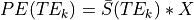
In the below equation,
.
In the below equation,  is signal at a given time
  and for a given echo time
  .
.
 is the mean signal across time for the echo time
.
is the mean signal across time for the echo time
.
 is the difference in at time from the average .
 is the difference in
  at time from the average .
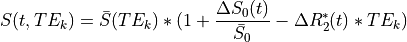
If we ignore time, this can be simplified to
In order to evaluate whether signal change is being driven by fluctuations in
either or , one can break this overall model
into submodels by zeroing out certain terms.
Important
Remember- is just 
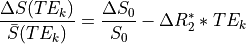
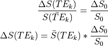
For a TE-independence model, if there were no fluctuations in :
Note that TE is not a parameter in this model. Hence, this model is TE-independent.
Also,  is a scalar (i.e., doesn’t change with
TE), so we can just ignore that, which means we only use
is a scalar (i.e., doesn’t change with
TE), so we can just ignore that, which means we only use  (mean echo-wise signal).
Thus, the model becomes 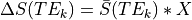 , where we
fit X to the data using regression and evaluate model fit.
, where we
fit X to the data using regression and evaluate model fit.
For TEDPCA/TEDICA, we use regression to get parameter estimates (raw PEs; not
standardized beta values) for component time-series against echo-specific data,
and substitute those PEs for .
Thus, to assess the TE-independence of a component, we use the model
 , fit X to the data, and evaluate model
fit.
, fit X to the data, and evaluate model
fit.
For a TE-dependence model, if there were no fluctuations in :
Note that TE is a parameter in this model. Hence, it is TE-dependent.
Applying our models to signal decay curves
As an example, let us simulate some data.
We will simulate signal decay for two time points, as well as the signal decay
for the hypothetical overall average over time.
In one time point, only will fluctuate.
In the other, only will fluctuate.
Caution
To make things easier, we’re simulating these data with echo times of 0 to
200 milliseconds, at 1ms intervals.
In real life, you’ll generally only have 3-5 echoes to work with.
Real signal from each echo will also be contaminated with random noise and
will have influences from both and .
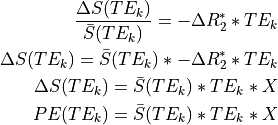
We can see that  has very different curves for the two
simulated datasets.
Moreover, as expected,
has very different curves for the two
simulated datasets.
Moreover, as expected,  is flat
across echoes for the -fluctuating data and scales roughly linearly with TE
for the -fluctuating data.
is flat
across echoes for the -fluctuating data and scales roughly linearly with TE
for the -fluctuating data.
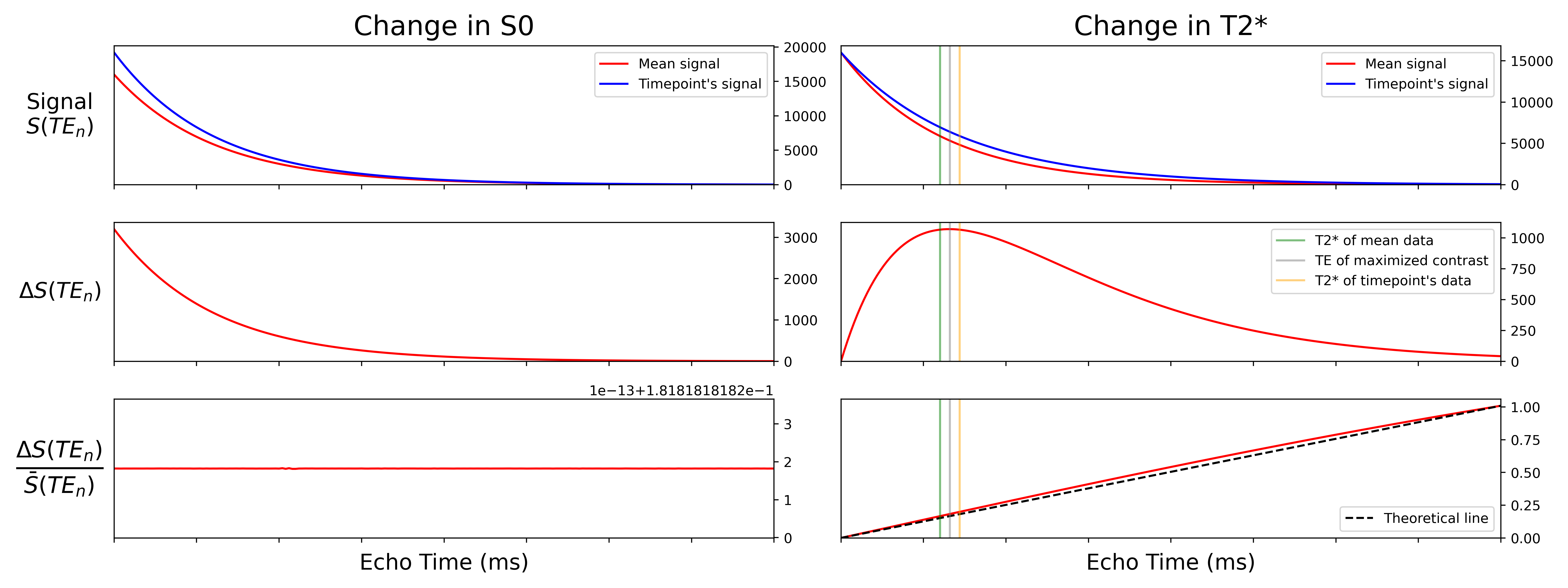
We then fit our TE-dependence and TE-independence models to the
data, which gives us predicted data for each model for
each dataset.
As expected, the model fits perfectly to the -fluctuating dataset, while
the model fits quite well to the -fluctuating dataset.
The actual model fits can be calculated as F-statistics. Then, the F-statistics per voxel are averaged across voxels into the Kappa and Rho pseudo-F-statistics.
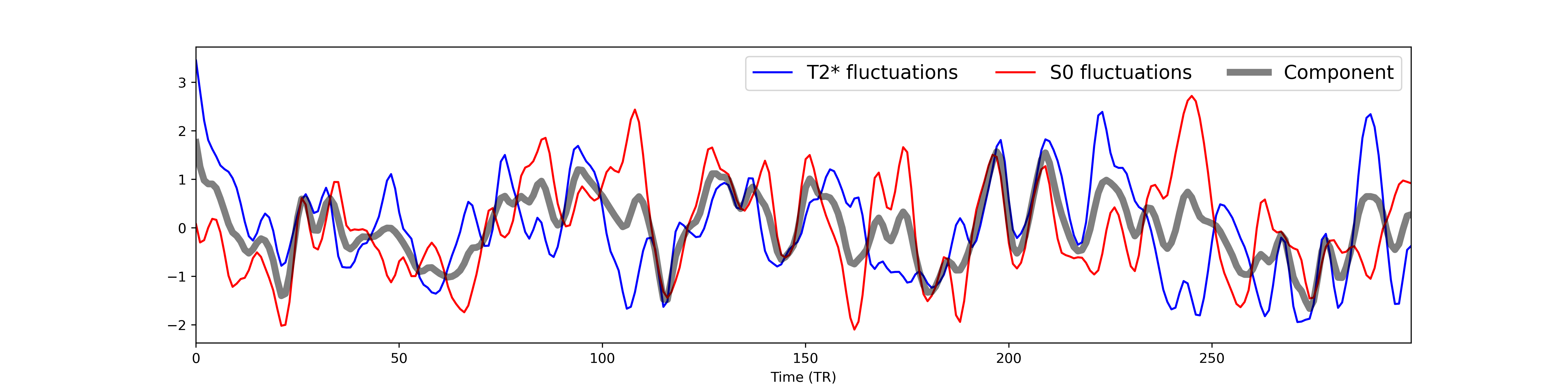
Applying our models to spatiotemporal decompositions
Now let us see how this extends to time series, components, and component parameter estimates.
We have the means to simulate - and -based fluctuations, so here we have
generated two time series- one -based and one -based.
Both time series share the same level of percent signal change (a standard
deviation equivalent to 5% of the mean), although the mean (16000) is very
different from the mean (30).
We can then average those two time series with different weights to create
components that are - or -based to various degrees.
In this case, both and contribute equally to the simulated time series.
This simulated time series will act as our ICA component for this example.
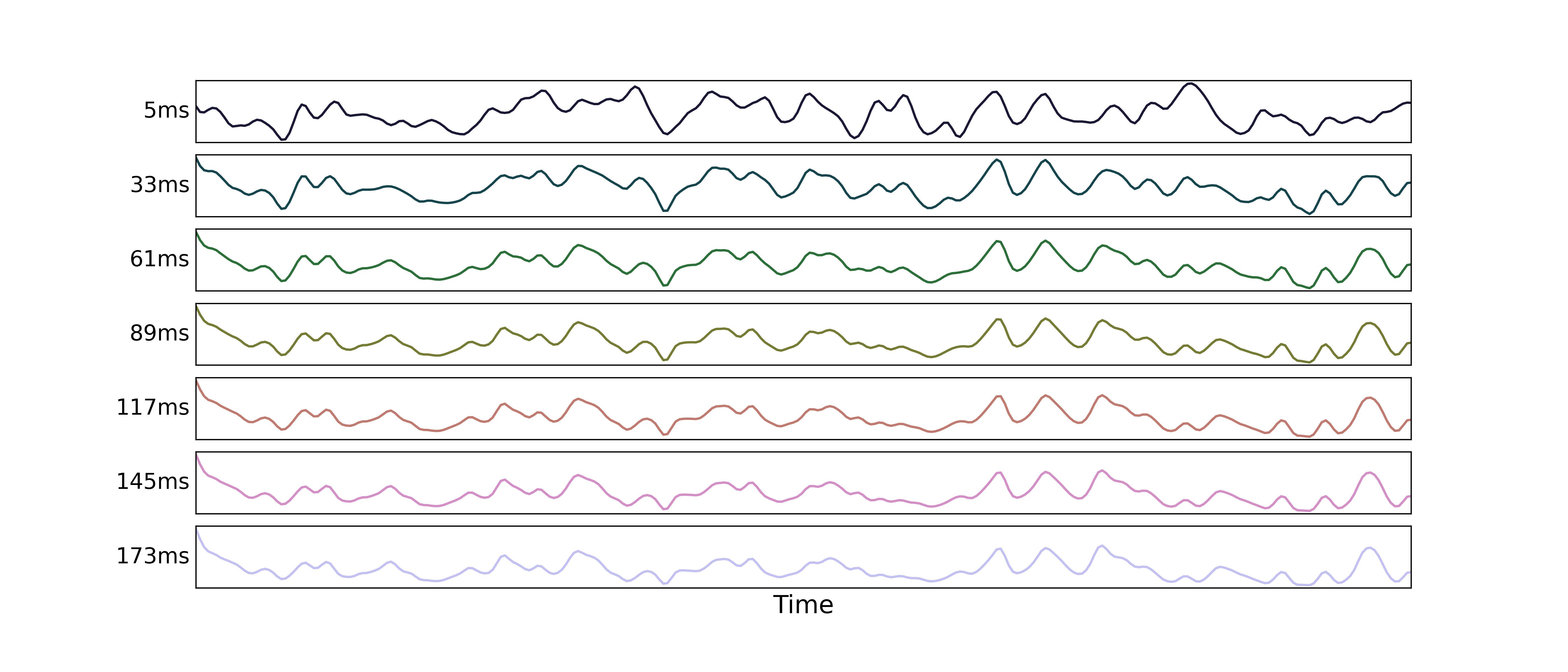
We also simulate multi-echo data for a single voxel with the same levels of
and fluctuations as in the pure and time series above.
Here we show time series for a subset of echo times.
And here we can see how those signals decay with echo time (again for only a subset of echo times):
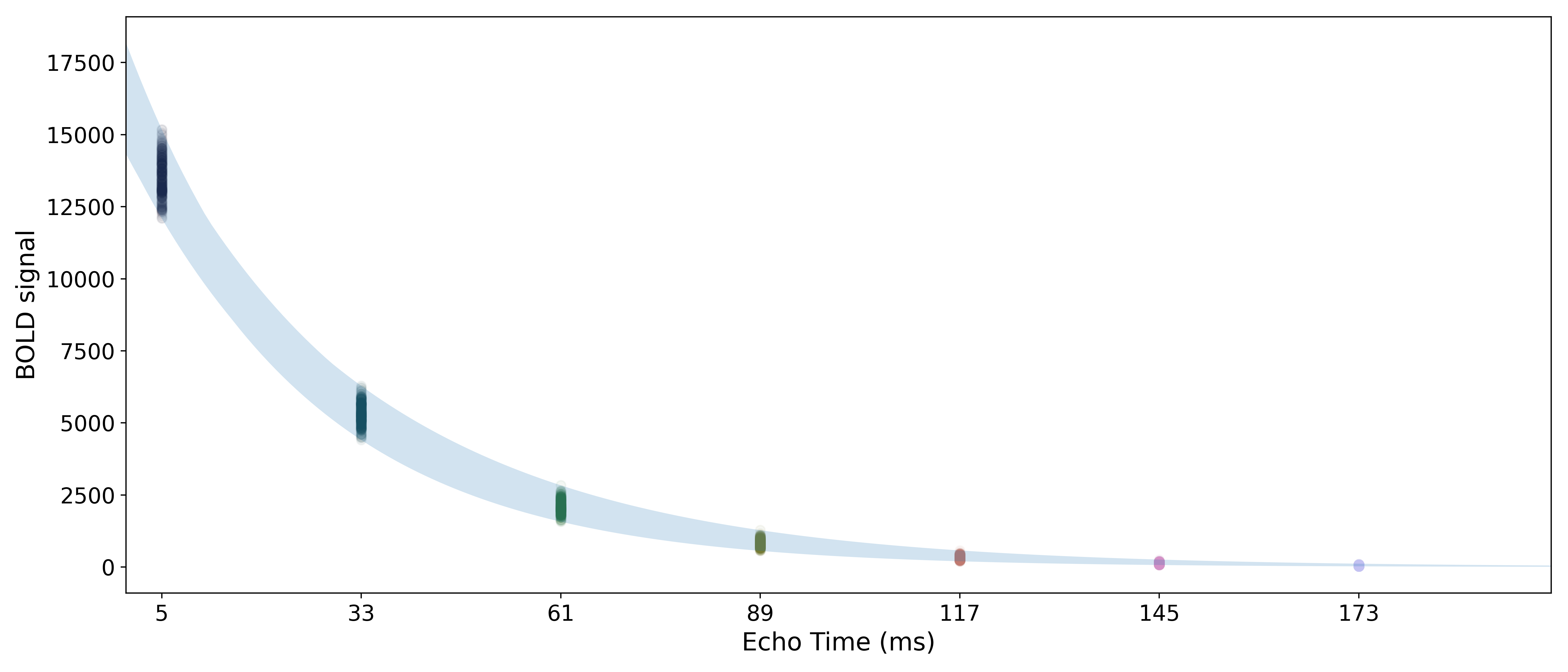
We then run a regression for each echo’s data against the component time series,
producing one parameter estimate for each echo time.
The parameter estimates match the signal decay curve for ,
as seen above.
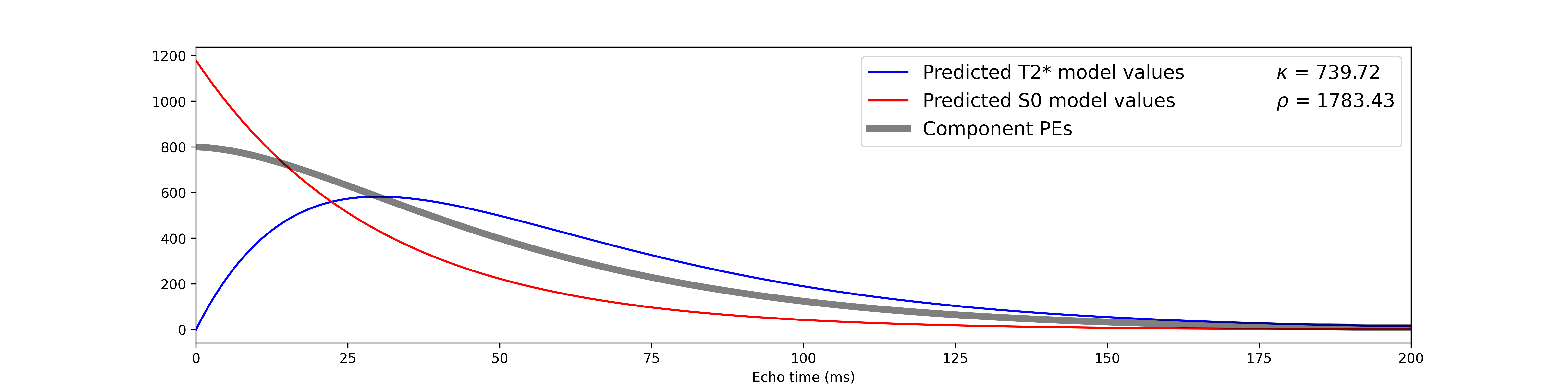
We can thus apply the same TE-dependence and -independence models as above,
in order to calculate single-voxel  and
and  values.
Note that the metric values are extremely high, due to the inflated
degrees of freedom resulting from using so many echoes in the simulations.
values.
Note that the metric values are extremely high, due to the inflated
degrees of freedom resulting from using so many echoes in the simulations.
Attention
You may also notice that, despite the fact that and fluctuate the same
amount and that both contributed equally to the component, is
much higher than .
Other Available Metrics
In addition to the core (in)dependence model metrics, TEDANA can also calculate the following metrics:
countnoise
tedana.metrics.dependence.compute_countnoise()
The number of significant voxels in each component’s standardized parameter estimate map that are not in clusters. In theory, these non-cluster voxels should be noise, and if a component exhibits more non-cluster voxels than cluster voxels, it is more likely to be noise.
countsigFT2
tedana.metrics.dependence.compute_countsignal()
The number of significant voxels in each component’s T2*-model F-statistic map that are in clusters. Having these “signal” voxels in the T2*-model F-statistic map is a good indicator that the component is signal, and having more cluster voxels in the S0-model F-statistic map than in the T2*-model F-statistic map is a good indicator that the component is noise.
countsigFS0
tedana.metrics.dependence.compute_countsignal()
The number of significant voxels in each component’s S0-model F-statistic map that are in clusters. Having more cluster voxels in the S0-model F-statistic map than in the T2*-model F-statistic map is a good indicator that the component is noise.
dice_FT2
tedana.metrics.dependence.compute_dice()
The Dice similarity index between each component’s cluster-extent thresholded T2*-model F-statistic map (using a p<0.05 threshold) and its cluster-extent thresholded standardized parameter estimate map (using a 5% threshold). This is a measure of the similarity between the T2*-model F-statistic map and the weight map. If the standardized parameter estimate map has a higher DSI with the T2*-model F-statistic map than the S0-model F-statistic map, it is more likely to be signal.
dice_FS0
tedana.metrics.dependence.compute_dice()
The Dice similarity index between each component’s cluster-extent thresholded S0-model F-statistic map (using a p<0.05 threshold) and its cluster-extent thresholded standardized parameter estimate map (using a 5% threshold). This is a measure of the similarity between the S0-model F-statistic map and the standardized parameter estimate map. If the standardized parameter estimate map has a higher DSI with the S0-model F-statistic map than the T2*-model F-statistic map, it is more likely to be noise.
signal-noise_t
tedana.metrics.dependence.compute_signal_minus_noise_t()
A t-test is performed between the distributions of unique T2*-model F-statistics
associated with clusters (i.e., signal) and non-cluster voxels (i.e., noise) to
generate a t-statistic (metric signal-noise_t) and p-value (metric signal-noise_p)
measuring relative association of the component to signal over noise.
signal-noise_z
tedana.metrics.dependence.compute_signal_minus_noise_z()
A t-test is performed between the distributions of T2*-model F-statistics
associated with clusters (i.e., signal) and non-cluster voxels (i.e., noise) to
generate a z-statistic (metric signal-noise_z) and p-value (metric signal-noise_p)
measuring relative association of the component to signal over noise.
This metric has not been used in the literature- the tedana developers created it
to address statistical issues with signal-noise_t
(e.g., the fact that signal-noise_t limits inputs to unique F-statistics
and it later applies thresholds appropriate for z-statistics to the t-statistics).
variance explained
tedana.metrics.dependence.calculate_varex()
The “variance explained” by each component is calculated as the square of the parameter estimates from the regression of the mean-centered, but not z-scored, optimally combined data against the component time series, divided by the sum of the squares of the parameter estimates.
Important
Please note that:
This is NOT variance explained (R^2).
Values sum to 100% by construction.
Shared variance among correlated components is implicitly distributed across coefficients in a model-dependent manner.
This metric reflects relative participation in the fitted model, not unique or marginal explanatory power.
This corresponds to the quantity historically referred to as “variance explained” in tedana, but is more accurately described as relative coefficient energy.
normalized variance explained
tedana.metrics.dependence.calculate_varex()
The “normalized variance explained” by each component is calculated as the square of the standardized parameter estimates from the regression of the z-scored optimally combined data against the z-scored component time series, divided by the sum of the squares of the standardized parameter estimates.
This is not actually a measure of normalized variance explained.
In the tedpca metrics, “normalized variance explained” actually comes from
the fitted PCA object’s explained_variance_ratio_ attribute,
and the TEDANA-calculated value is retained as “estimated normalized variance explained”.
marginal R-squared
tedana.metrics.dependence.calculate_marginal_r2()
The “marginal R-squared” by each component is calculated as 100 times the squared correlation between the component time series and the data, averaged over voxels.
This represents the variance in the data explained by each component without controlling for other components.
partial R-squared
tedana.metrics.dependence.calculate_partial_r2()
The “partial R-squared” by each component is calculated as the proportion (expressed as a percentage) of variance uniquely explained by that component relative to the sum of this uniquely explained variance and the variance that is not explained by the full model.
This is equivalent to the variance explained by each component after regressing the other components out of the data and the component itself. It is a conditional effect size.
semi-partial R-squared
tedana.metrics.dependence.calculate_semipartial_r2()
The “semi-partial R-squared” by each component is computed by first orthogonalizing that component with respect to all other components (i.e., regressing it onto the remaining components and taking the residuals). The squared Pearson correlation between this orthogonalized regressor and the data is then computed for each voxel, and the semi-partial R-squared for that component is the mean of these squared correlations across voxels.
This corresponds to the variance in the data that is uniquely explained by each component, after removing variance that is shared with the other components. It indicates the incremental increase in R-squared when adding the target component to the model.
kappa_rho_difference
tedana.metrics.dependence.compute_kappa_rho_difference()
The difference between the kappa and rho metrics is calculated as the absolute value of the difference between the kappa and rho metrics divided by the sum of the kappa and rho metrics.
Higher values indicate that the component is more dominated by either kappa or rho, which indicates “specificity” of the component to either TE-dependent or TE-independent signals.
d_table_score
tedana.metrics.dependence.generate_decision_table_score()
A five-metric decision table is generated by ranking a number of metrics in either descending or ascending order if they measure TE-dependence or TE-independence, respectively, and then averaging the ranks. The metrics are: - kappa - dice_FT2 - signal-noise_t - countnoise - countsigFT2
The decision table score is then calculated as the average of the ranks of the metrics.