Outputs of tedana

Outputs of the tedana workflow

Filename	Content
dataset_description.json	Top-level metadata for the workflow.
T2starmap.nii.gz	Full estimated T2* 3D map. Values are in seconds. The difference between the limited and full maps is that, for voxels affected by dropout where only one echo contains good data, the full map uses the T2* estimate from the first two echoes, while the limited map has a NaN.
S0map.nii.gz	Full S0 3D map. The difference between the limited and full maps is that, for voxels affected by dropout where only one echo contains good data, the full map uses the S0 estimate from the first two echoes, while the limited map has a NaN.
desc-optcom_bold.nii.gz	Optimally combined time series.
desc-optcomDenoised_bold.nii.gz	Denoised optimally combined time series. Recommended dataset for analysis.
desc-optcomRejected_bold.nii.gz	Combined time series from rejected components.
desc-optcomAccepted_bold.nii.gz	High-kappa time series. This dataset does not include thermal noise or low variance components. Not the recommended dataset for analysis.
desc-adaptiveGoodSignal_mask.nii.gz	Integer-valued mask used in the workflow, where each voxel’s value corresponds to the number of good echoes to be used for T2*/S0 estimation.
desc-PCA_mixing.tsv	Mixing matrix (component time series) from PCA decomposition in a tab-delimited file. Each column is a different component, and the column name is the component number.
desc-PCA_decomposition.json	Metadata for the PCA decomposition.
desc-PCA_stat-z_components.nii.gz	Component weight maps from PCA decomposition. Each map corresponds to the same component index in the mixing matrix and component table. Maps are in z-statistics.
desc-PCA_metrics.tsv	TEDPCA component table. A BIDS Derivatives-compatible TSV file with summary metrics and inclusion/exclusion information for each component from the PCA decomposition.
desc-PCA_metrics.json	Metadata about the metrics in desc-PCA_metrics.tsv.
desc-ICA_mixing.tsv	Mixing matrix (component time series) from ICA decomposition in a tab-delimited file. Each column is a different component, and the column name is the component number.
desc-ICA_components.nii.gz	Full ICA coefficient feature set.
desc-ICA_stat-z_components.nii.gz	Z-statistic component weight maps from ICA decomposition. Values are z-transformed standardized regression coefficients. Each map corresponds to the same component index in the mixing matrix and component table.
desc-ICA_decomposition.json	Metadata for the ICA decomposition.
desc-tedana_metrics.tsv	TEDICA component table. A BIDS Derivatives-compatible TSV file with summary metrics and inclusion/exclusion information for each component from the ICA decomposition.
desc-tedana_metrics.json	Metadata about the metrics in desc-tedana_metrics.tsv.
desc-ICAAccepted_components.nii.gz	High-kappa ICA coefficient feature set
desc-ICAAcceptedZ_components.nii.gz	Z-normalized spatial component maps
report.txt	A summary report for the workflow with relevant citations.
tedana_report.html	The interactive HTML report.

If verbose is set to True:

Filename	Content
desc-limited_T2starmap.nii.gz	Limited T2* map/time series. Values are in seconds. The difference between the limited and full maps is that, for voxels affected by dropout where only one echo contains good data, the full map uses the S0 estimate from the first two echoes, while the limited map has a NaN.
desc-limited_S0map.nii.gz	Limited S0 map/time series. The difference between the limited and full maps is that, for voxels affected by dropout where only one echo contains good data, the full map uses the S0 estimate from the first two echoes, while the limited map has a NaN.
echo-[echo]_desc-[PCA|ICA]_components.nii.gz	Echo-wise PCA/ICA component weight maps.
echo-[echo]_desc-[PCA|ICA]R2ModelPredictions_components.nii.gz	Component- and voxel-wise R2-model predictions, separated by echo.
echo-[echo]_desc-[PCA|ICA]S0ModelPredictions_components.nii.gz	Component- and voxel-wise S0-model predictions, separated by echo.
desc-[PCA|ICA]AveragingWeights_components.nii.gz	Component-wise averaging weights for metric calculation.
desc-optcomPCAReduced_bold.nii.gz	Optimally combined data after dimensionality reduction with PCA. This is the input to the ICA.
echo-[echo]_desc-Accepted_bold.nii.gz	High-Kappa time series for echo number echo
echo-[echo]_desc-Rejected_bold.nii.gz	Low-Kappa time series for echo number echo
echo-[echo]_desc-Denoised_bold.nii.gz	Denoised time series for echo number echo

If gscontrol includes ‘gsr’:

Filename	Content
desc-globalSignal_map.nii.gz	Spatial global signal
desc-globalSignal_timeseries.tsv	Time series of global signal from optimally combined data.
desc-optcomWithGlobalSignal_bold.nii.gz	Optimally combined time series with global signal retained.
desc-optcomNoGlobalSignal_bold.nii.gz	Optimally combined time series with global signal removed.

If gscontrol includes ‘t1c’:

Filename	Content
desc-T1likeEffect_min.nii.gz	T1-like effect
desc-optcomAcceptedT1cDenoised_bold.nii.gz	T1-corrected high-kappa time series by regression
desc-optcomT1cDenoised_bold.nii.gz	T1-corrected denoised time series
desc-TEDICAAcceptedT1cDenoised_components.nii.gz	T1-GS corrected high-kappa components
desc-TEDICAT1cDenoised_mixing.tsv	T1-GS corrected mixing matrix

Component tables

TEDPCA and TEDICA use component tables to track relevant metrics, component classifications, and rationales behind classifications. The component tables are stored as tsv files for BIDS-compatibility.

In order to make sense of the rationale codes in the component tables, consult the tables below. TEDPCA rationale codes start with a “P”, while TEDICA codes start with an “I”.

Classification	Description
accepted	BOLD-like components included in denoised and high-Kappa data
rejected	Non-BOLD components excluded from denoised and high-Kappa data
ignored	Low-variance components included in denoised, but excluded from high-Kappa data

TEDPCA codes

Code	Classification	Description
P001	rejected	Low Rho, Kappa, and variance explained
P002	rejected	Low variance explained
P003	rejected	Kappa equals fmax
P004	rejected	Rho equals fmax
P005	rejected	Cumulative variance explained above 95% (only in stabilized PCA decision tree)
P006	rejected	Kappa below fmin (only in stabilized PCA decision tree)
P007	rejected	Rho below fmin (only in stabilized PCA decision tree)

TEDICA codes

Code	Classification	Description
I001	rejected|accepted	Manual classification
I002	rejected	Rho greater than Kappa
I003	rejected	More significant voxels in S0 model than R2 model
I004	rejected	S0 Dice is higher than R2 Dice and high variance explained
I005	rejected	Noise F-value is higher than signal F-value and high variance explained
I006	ignored	No good components found
I007	rejected	Mid-Kappa component
I008	ignored	Low variance explained
I009	rejected	Mid-Kappa artifact type A
I010	rejected	Mid-Kappa artifact type B
I011	ignored	ign_add0
I012	ignored	ign_add1

ICA Components Report

The reporting page for the tedana decomposition presents a series of interactive plots designed to help you evaluate the quality of your analyses. This page describes the plots forming the reports and well as information on how to take advantage of the interactive functionalities. You can also play around with our demo.

Report Structure

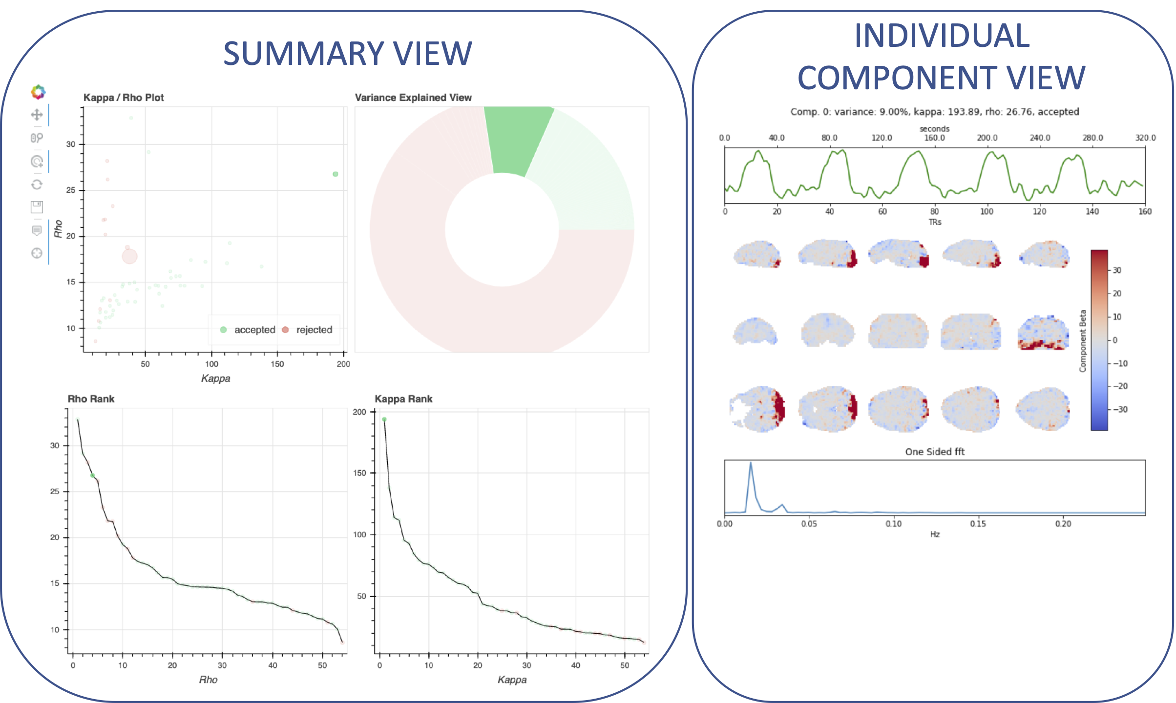
The image below shows a representative report, which has two sections: a) the summary view, and b) the individual component view.

Note

When a report is initially loaded, as no component is selected on the summary view, the individual component view appears empty.

Summary View

This view provides an overview of the decomposition and component selection results. It includes four different plots.

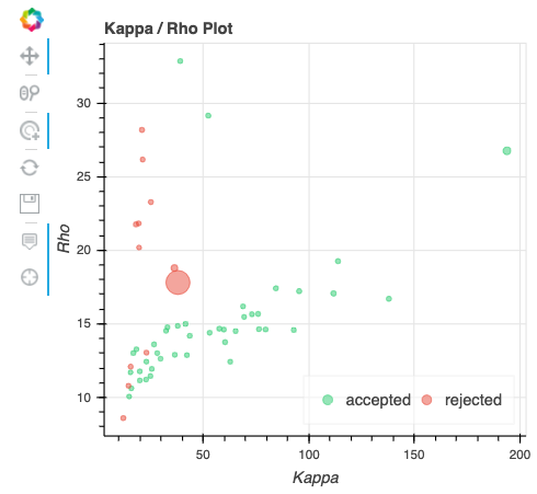
• Kappa/Rho Scatter: This is a scatter plot of Kappa vs. Rho features for all components. In the plot, each dot represents a different component. The x-axis represents the kappa feature, and the y-axis represents the rho feature. These are two of the most informative features describing the likelihood of the component being BOLD or non-BOLD. Additional information is provided via color and size. In particular, color informs about its classification status (e.g., accepted, rejected); while size relates to the amount of variance explained by the component (larger dot, larger variance).

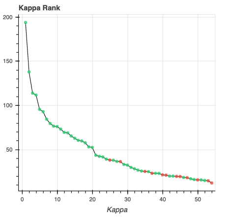
• Kappa Scree Plot: This scree plot provides a view of the components ranked by Kappa. As in the previous plot, each dot represents a component. The color of the dot informs us about classification status. In this plot, size is not related to variance explained.

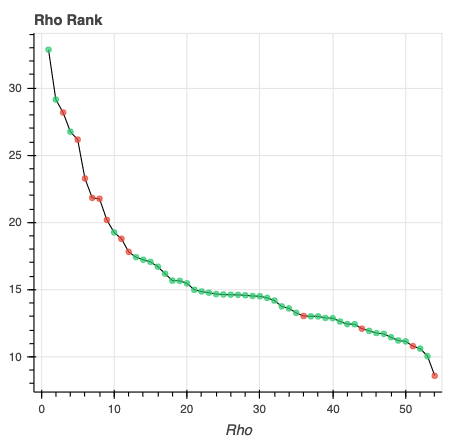
• Rho Scree Plot: This scree plot provides a view of the components ranked by Rho. As in the previous plot, each dot represents a component. The color of the dot informs us about classification status. In this plot, size is not related to variance explained.

• Variance Explained Plot: This pie plot provides a summary of how much variance is explained by each individual component, as well as the total variance explained by each of the three classification categories (i.e., accepted, rejected, ignored). In this plot, each component is represented as a wedge, whose size is directly related to the amount of variance explained. The color of the wedge inform us about the classification status of the component. For this view, components are sorted by classification first, and inside each classification group by variance explained.

Individual Component View

This view provides detailed information about an individual component (selected in the summary view, see below). It includes three different plots.

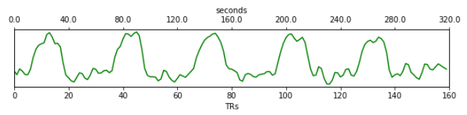
• Time series: This plot shows the time series associated with a given component (selected in the summary view). The x-axis represents time (in units of TR), and the y-axis represents signal levels (in arbitrary units). Finally, the color of the trace informs us about the component classification status.

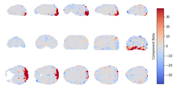
• Component beta map: This plot shows the map of the beta coefficients associated with a given component (selected in the summary view). The colorbar represents the amplitude of the beta coefficients.

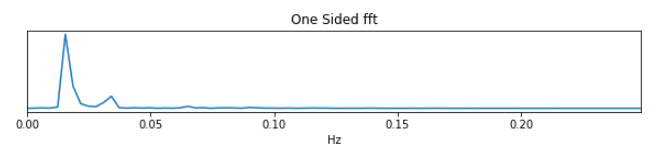
• Spectrum: This plot shows the spectrogram associated with a given component (selected in the summary view). The x-axis represents frequency (in Hz), and the y-axis represents spectral amplitude.

Reports User Interactions

As previously mentioned, all summary plots in the report allow user interactions. While the Kappa/Rho Scatter plot allows full user interaction (see the toolbar that accompanies the plot and the example below), the other three plots allow the user to select components and update the figures.

The table below includes information about all available interactions

Interaction	Icon	Description
Reset		Resets the data bounds of the plot to their values when the plot was initially created.
Wheel Zoom		Zoom the plot in and out, centered on the current mouse location.
Box Zoom		Define a rectangular region of a plot to zoom to by dragging the mouse over the plot region.
Crosshair		Draws a crosshair annotation over the plot, centered on the current mouse position
Pan		Allows the user to pan a plot by left-dragging a mouse across the plot region.
Hover		If active, the plot displays informational tooltips whenever the cursor is directly over a plot element.
Selection		Allows user to select components by tapping on the dot or wedge that represents them. Once a component is selected, the plots forming the individual component view update to show component specific information.
Save		Saves an image reproduction of the plot in PNG format.

Note

Specific user interactions can be switched on/off by clicking on their associated icon within the toolbar of a given plot. Active interactions show an horizontal blue line underneath their icon, while inactive ones lack the line.

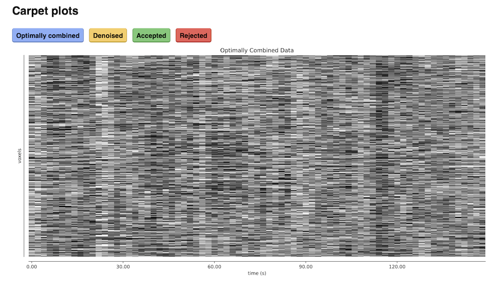
Carpet plots

In additional to the elements described above, tedana’s interactive reports include carpet plots for the main outputs of the workflow: the optimally combined data, the denoised data, the high-Kappa (accepted) data, and the low-Kappa (rejected) data.

These plots may be useful for visual quality control of the overall denoising run.

Citable workflow summaries

tedana generates a report for the workflow, customized based on the parameters used and including relevant citations. The report is saved in a plain-text file, report.txt, in the output directory.

An example report

TE-dependence analysis was performed on input data. An initial mask was generated from the first echo using nilearn’s compute_epi_mask function. An adaptive mask was then generated, in which each voxel’s value reflects the number of echoes with ‘good’ data. A monoexponential model was fit to the data at each voxel using nonlinear model fitting in order to estimate T2* and S0 maps, using T2*/S0 estimates from a log-linear fit as initial values. For each voxel, the value from the adaptive mask was used to determine which echoes would be used to estimate T2* and S0. In cases of model fit failure, T2*/S0 estimates from the log-linear fit were retained instead. Multi-echo data were then optimally combined using the T2* combination method (Posse et al., 1999). Principal component analysis in which the number of components was determined based on a variance explained threshold was applied to the optimally combined data for dimensionality reduction. A series of TE-dependence metrics were calculated for each component, including Kappa, Rho, and variance explained. Independent component analysis was then used to decompose the dimensionally reduced dataset. A series of TE-dependence metrics were calculated for each component, including Kappa, Rho, and variance explained. Next, component selection was performed to identify BOLD (TE-dependent), non-BOLD (TE-independent), and uncertain (low-variance) components using the Kundu decision tree (v2.5; Kundu et al., 2013). Rejected components’ time series were then orthogonalized with respect to accepted components’ time series.

This workflow used numpy (Van Der Walt, Colbert, & Varoquaux, 2011), scipy (Jones et al., 2001), pandas (McKinney, 2010), scikit-learn (Pedregosa et al., 2011), nilearn, and nibabel (Brett et al., 2019).

This workflow also used the Dice similarity index (Dice, 1945; Sørensen, 1948).

References

Brett, M., Markiewicz, C. J., Hanke, M., Côté, M.-A., Cipollini, B., McCarthy, P., … freec84. (2019, May 28). nipy/nibabel. Zenodo. http://doi.org/10.5281/zenodo.3233118

Dice, L. R. (1945). Measures of the amount of ecologic association between species. Ecology, 26(3), 297-302.

Jones E, Oliphant E, Peterson P, et al. SciPy: Open Source Scientific Tools for Python, 2001-, http://www.scipy.org/

Kundu, P., Brenowitz, N. D., Voon, V., Worbe, Y., Vértes, P. E., Inati, S. J., … & Bullmore, E. T. (2013). Integrated strategy for improving functional connectivity mapping using multiecho fMRI. Proceedings of the National Academy of Sciences, 110(40), 16187-16192.

McKinney, W. (2010, June). Data structures for statistical computing in python. In Proceedings of the 9th Python in Science Conference (Vol. 445, pp. 51-56).

Pedregosa, F., Varoquaux, G., Gramfort, A., Michel, V., Thirion, B., Grisel, O., … & Vanderplas, J. (2011). Scikit-learn: Machine learning in Python. Journal of machine learning research, 12(Oct), 2825-2830.

Posse, S., Wiese, S., Gembris, D., Mathiak, K., Kessler, C., Grosse‐Ruyken, M. L., … & Kiselev, V. G. (1999). Enhancement of BOLD‐contrast sensitivity by single‐shot multi‐echo functional MR imaging. Magnetic Resonance in Medicine: An Official Journal of the International Society for Magnetic Resonance in Medicine, 42(1), 87-97.

Sørensen, T. J. (1948). A method of establishing groups of equal amplitude in plant sociology based on similarity of species content and its application to analyses of the vegetation on Danish commons. I kommission hos E. Munksgaard.

Van Der Walt, S., Colbert, S. C., & Varoquaux, G. (2011). The NumPy array: a structure for efficient numerical computation. Computing in Science & Engineering, 13(2), 22.