ICA Components Report¶

The reporting page for the tedana decomposition presents a series of interactive plots designed to help you evaluate the quality of your analyses. This page describes the plots forming the reports and well as information on how to take advantage of the interactive functionalities. You can also play around with our demo.

Report Structure¶

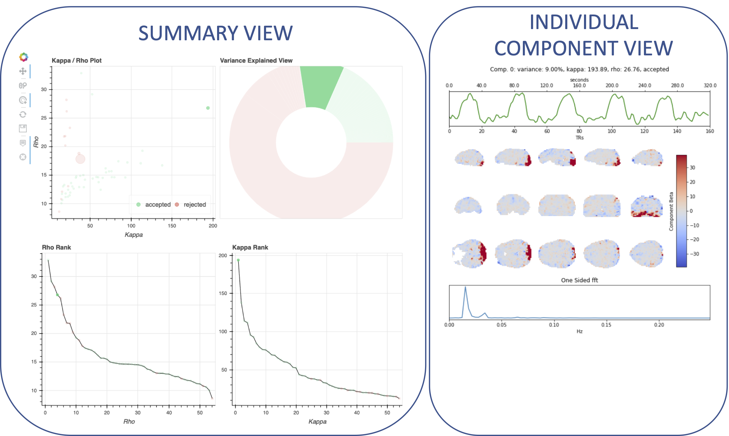
The image below shows a representative report, which has two sections: a) the summary view, and b) the individual component view.

Note

When a report is initially loaded, as no component is selected on the summary view, the individual component view appears empty.

Summary View¶

This view provides an overview of the decomposition and component selection results. It includes four different plots.

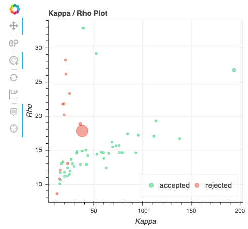
Kappa/Rho Scatter: This is a scatter plot of Kappa vs. Rho features for all components. In the plot, each dot represents a different component. The x-axis represents the kappa feature, and the y-axis represents the rho feature. These are two of the most informative features describing the likelihood of the component being BOLD or non-BOLD. Additional information is provided via color and size. In particular, color informs about its classification status (e.g., accepted, rejected); while size relates to the amount of variance explained by the component (larger dot, larger variance).

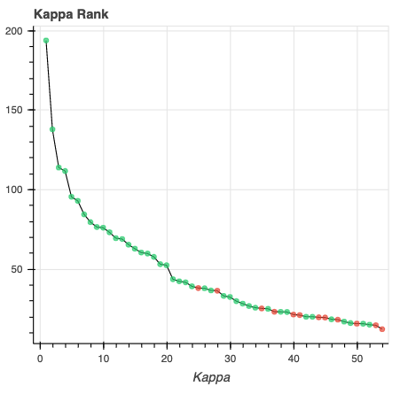
Kappa Scree Plot: This scree plot provides a view of the components ranked by Kappa. As in the previous plot, each dot represents a component. The color of the dot informs us about classification status. In this plot, size is not related to variance explained.

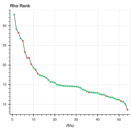
Rho Scree Plot: This scree plot provides a view of the components ranked by Rho. As in the previous plot, each dot represents a component. The color of the dot informs us about classification status. In this plot, size is not related to variance explained.

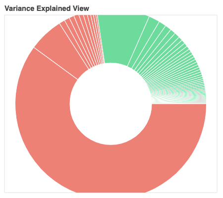
Variance Explained Plot: This pie plot provides a summary of how much variance is explained by each individual component, as well as the total variance explained by each of the three classification categories (i.e., accepted, rejected, ignored). In this plot, each component is represented as a wedge, whose size is directly related to the amount of variance explained. The color of the wedge inform us about the classification status of the component. For this view, components are sorted by classification first, and inside each classification group by variance explained.

Individual Component View¶

This view provides detailed information about an individual component (selected in the summary view, see below). It includes three different plots.

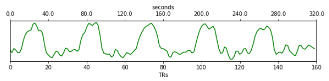
Time series: This plot shows the time series associated with a given component (selected in the summary view). The x-axis represents time (in units of TR), and the y-axis represents signal levels (in arbitrary units). Finally, the color of the trace informs us about the component classification status.

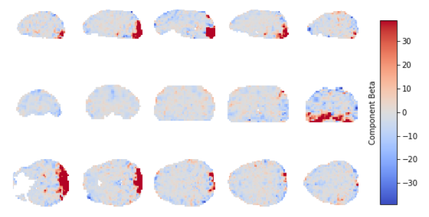
Component beta map: This plot shows the map of the beta coefficients associated with a given component (selected in the summary view). The colorbar represents the amplitude of the beta coefficients.

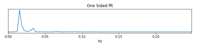
Spectrum: This plot shows the spectrogram associated with a given component (selected in the summary view). The x-axis represents frequency (in Hz), and the y-axis represents spectral amplitude.

Reports User Interactions¶

As previously mentioned, all summary plots in the report allow user interactions. While the Kappa/Rho Scatter plot allows full user interaction (see the toolbar that accompanies the plot and the example below), the other three plots allow the user to select components and update the figures.

The table below includes information about all available interactions

Interaction	Icon	Description
Reset		Resets the data bounds of the plot to their values when the plot was initially created.
Wheel Zoom		Zoom the plot in and out, centered on the current mouse location.
Box Zoom		Define a rectangular region of a plot to zoom to by dragging the mouse over the plot region.
Crosshair		Draws a crosshair annotation over the plot, centered on the current mouse position
Pan		Allows the user to pan a plot by left-dragging a mouse across the plot region.
Hover		If active, the plot displays informational tooltips whenever the cursor is directly over a plot element.
Selection		Allows user to select components by tapping on the dot or wedge that represents them. Once a component is selected, the plots forming the individual component view update to show component specific information.
Save		Saves an image reproduction of the plot in PNG format.

Note

Specific user interactions can be switched on/off by clicking on their associated icon within the toolbar of a given plot. Active interactions show an horizontal blue line underneath their icon, while inactive ones lack the line.